NMM project: motion planner

This project is an exploration of solving trajectory motion planning as a constrained optimization, taking into account speed, acceleration and jerk constraints, including effects that depend on the current speed itself.

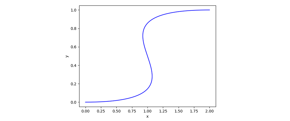
To avoid dealing with the initially unknown time dynamics, we solve the problem in the phase space, where time is implicitly defined from the current speed and position. Here is a sneak peek of the solver finding a jerk-limited S-curve for a simple 1D motion

1D motion

Problem statement

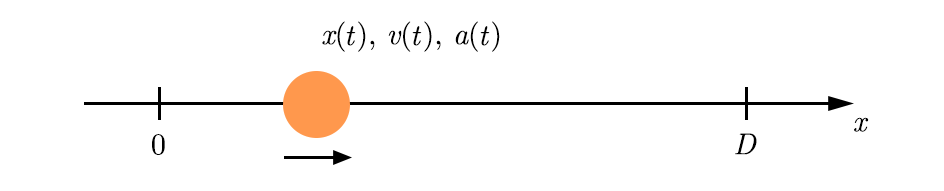
Let’s simply assume a moving mass on a 1D axis. We want to solve the time trajectory $x(t)$ given a start and end positions $x(0)=0$ and $x(T)=D$, where $T$ is the total travel time.

We can define the speed $v=\frac{{\rm d} x}{{\rm d} t}$ and acceleration $a=\frac{{\rm d}^2 x}{{\rm d} t^2}$. We can also define the jerk $j=\frac{{\rm d} a}{{\rm d} t}=\frac{{\rm d}^3 x}{{\rm d} t^3}$. Limiting the jerk prevents instant changes in acceleration, which are a known issue that causes shaking on heavier machines.

We want to solve $x(t)$ and figure out $T$ given:

• Speed constraints: $$|v| \leq v_{\rm max}$$
• Acceleration constraints: $$a_{\rm min} \leq a \leq a_{\rm max}$$
• Jerk constraints: $$|j| \leq j_{\rm max}$$

Note that $a_{\rm min}$ and $a_{\rm max}$ are not necessarily constant: real machines have limited force as a function of the current speed $v$. We’ll explore this generalized case in the next sections.

The initial/final conditions are:

• $x(0)=0$, $x(T)=D$
• $v(0)=0$, $v(T)=0$
• $a(0)=0$, $a(T)=0$

Phase space representation

The issue with solving $x$, $v$ and $a$ in the time domain is that the time function is itself a function of the dynamics.

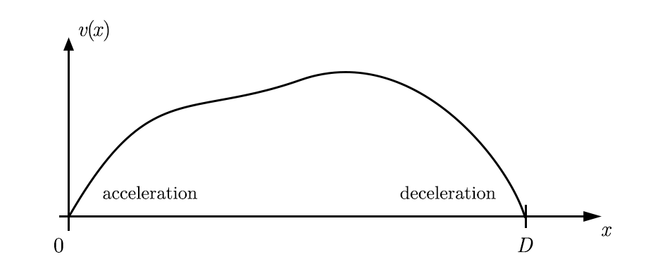
We instead choose to solve $v$ and $a$ as functions of $x$ in a phase space model:

In that representation, time is implicit and has a deep relation to the $x, v$ curve:

$$v=\frac{{\rm d} x}{{\rm d} t} \Rightarrow {\rm d} t=\frac{{\rm d} x}{v}$$

The travel time can be found through integration:

$$t=\int_0^x \frac{{\rm d} x}{v(x)}$$

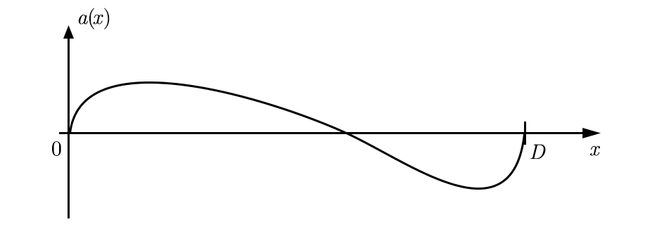
The total travel time is found by taking this integral up to $x=D$. The acceleration can be found from $v(x)$ as follows:

$$a(x)=\frac{{\rm d} v(x)}{{\rm d} t}=\frac{{\rm d} v(x)}{{\rm d} x} \frac{{\rm d} x}{{\rm d} t}=v'(x)v(x)$$

Note that this is only valid for non-zero $v(x)$, which is the case over the inner domain of the problem $x~\in~]0, D[$. For the previous speed curve, this might look something like this:

The problem can now be formulated as a search for a $v(x)$ curve that has the following properties:

• Minimize $$T=\int_0^D \frac{{\rm d} x}{v(x)}$$
• Subject to:
  • $|v(x)| \leq v_{\rm max}~\forall x \in~[0, D]$
  • $a_{\rm min} \leq a(x) \leq a_{\rm max}~\forall x \in~[0, D]$
  • $|j(x)| < j_{\rm max}~\forall x \in~[0, D]$
  • $v(0)=v(D)=0$
  • $a(0)=a(D)=0$

We’ll follow the intuition that $v(x)$ has to be “inflated” as much as can be, until the constraints are touched for every $x$.

Discrete solver

Instead of tackling the continuous problem, we can discretize $x(k)$ and solve a discrete vector $v(k)$, with $k=0\dots N-1$. We define a time increment by using the mean speed over a segment:

$$\Delta t (k) = \frac{\Delta x(k)}{v_{\rm mean}(k)} = \frac{x(k+1)-x(k)}{0.5(v(k+1) + v(k))}$$

As long as no two sequential values of $v(k)$ are zero, $\Delta t$ is always defined. Given accelerations limits over a segment, we can define cones of possible values for future and past speeds:

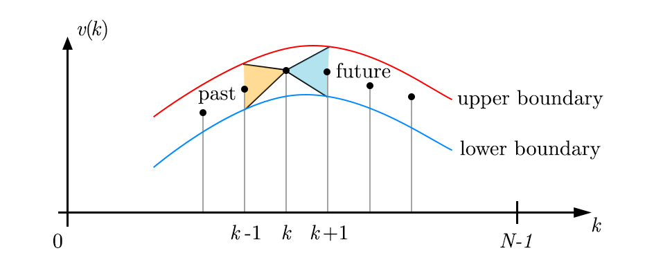
Note that the existence of this cone is merely an artifact of the discretization of time, but we can use it to our advantage. Accelerations are subject to a similar

Here is a naive but effective approach to solve our problem:

1. Start with a small value for $v(k), k \in [1, N-2]$.
2. Evaluate acceleration $a(k)$ from $v(k)$.
3. Given jerk and acceleration constraints, compute horizons $a_{\rm min}(k)$ and $a_{\rm max}(k)$ for each segment.
4. Given $a_{\rm min}(k)$ and $a_{\rm max}(k)$ and speed limit, evaluate horizons $v_{\rm min}(k)$ and $v_{\rm max}(k)$ for each point.
5. Update $v(k) \Rightarrow \lambda v_{\rm max} + (1-\lambda) v$
6. Repeat steps 2-5 until $|v_{\rm max}(k) - v(k)|_2 < \epsilon$

Let’s implement step 3:

def constraint_a(x, v, acc_model, jerk_max, a_start=None, a_end=None):
    """
    inputs: position vector x, speed vector v
    returns: min. and max. acceleration for each segment
    """
    dx = x[1:] - x[:-1]
    x_mid = (x[:-1] + x[1:]) * 0.5
    v_mid = (v[:-1] + v[1:]) * 0.5
    dt = dx / v_mid
    a = (v[1:] - v[:-1]) / t_delta
    dt_a = (dt[:-1] + dt[1:]) * 0.5

    a_max_next = a[:-1] + jerk_max * dt_a 
    a_min_next = a[:-1] - jerk_max * dt_a 
    a_max_prev = a[1:] + jerk_max * dt_a 
    a_min_prev = a[1:] - jerk_max * dt_a 
    a_min = np.zeros_like(a)
    a_max = np.zeros_like(a)

    if a_start is None:
        a_min[0] = a_min_prev[0]
        a_max[0] = a_max_prev[0]
    else:
        # constrain end acceleration
        a_max[0] = a_start + jerk_max * t_delta_a[0]
        a_min[0] = a_start - jerk_max * t_delta_a[0]

    if a_end is None:
        a_min[-1] = a_min_next[-1]
        a_max[-1] = a_max_next[-1]
    else:
        # constrain end acceleration
        a_max[-1] = a_end + jerk_max * t_delta_a[-1]
        a_min[-1] = a_end - jerk_max * t_delta_a[-1]

    a_min[1:-1] = np.maximum(a_min_next[:-1], a_min_prev[1:])
    a_max[1:-1] = np.minimum(a_max_next[:-1], a_max_prev[1:])

    a_neg_bound, a_pos_bound = acc_model(v_mid)
    a_min = np.maximum(a_min, a_neg_bound)
    a_max = np.minimum(a_max, a_pos_bound)
    a_min = np.minimum(a_min, a)
    a_max = np.maximum(a_max, a)

    return a_min, a_max

Step 4 is similar:

def constraint_v(x, v, a_min, a_max, v_abs_max, v_start=None, v_end=None):
    """
    inputs: position vector x, speed vector v
    returns: min. and max. speed for each segment
    """
    dx = x[1:] - x[:-1]
    v_mid = (v[:-1] + v[1:]) * 0.5
    dt = dx / v_mid

    v_max_next = v[:-1] + a_max * dt
    v_min_next = v[:-1] + a_min * dt
    v_max_prev = v[1:] - a_min * dt
    v_min_prev = v[1:] - a_max * dt
    v_min = np.zeros_like(v)
    v_max = np.zeros_like(v)
    if v_start is None:
        v_max[0] = v_max_prev[0]
        v_min[0] = v_min_prev[0]
    else:
        # constrain start speed
        v_max[0] = v_start
        v_min[0] = v_start

    if v_end is None:
        v_max[-1] = v_max_next[-1]
        v_min[-1] = v_min_next[-1]
    else:
        # constrain end speed
        v_max[-1] = v_end
        v_min[-1] = v_end

    v_min[1:-1] = np.maximum(v_min_next[:-1], v_min_prev[1:])
    v_max[1:-1] = np.minimum(v_max_next[:-1], v_max_prev[1:])
    v_min = np.maximum(v_min, -v_abs_max)
    v_max = np.minimum(v_max, v_abs_max)

    return v_min, v_max

Now we can put it all together:

# acceleration horizon
a_min, a_max = constraint_a(x, v, acc_model_simple, jerk_max)

# speed horizon
v_min, v_max = constraint_v(x, v, a_min, a_max)

# update
v[:] = v_max * lambd + v * (1 - lambd)

It turns the whole method can be unstable if $\lambda$ is too optimistic. One big flaw of the method is that modifying $v$ also changes the duration of a step. Ignoring this can lead to invalid speed horizons in step 4. We can improve this using an updated estimate of $\Delta t$ and solving for $v$:

def constraint_v(x, v, a_min, a_max, v_abs_max, v_start=None, v_end=None):
    """
    inputs: position vector x, speed vector v
    returns: min. and max. speed for each segment
    """
    dx = x[1:] - x[:-1]
    
    v_max_next = np.sqrt(np.maximum(v[:-1]**2 + 2 * a_max * dx, 0))
    v_min_next = np.sqrt(np.maximum(v[:-1]**2 + 2 * a_min * dx, 0))
    v_min_prev = np.sqrt(np.maximum(v[1:]**2 - 2 * a_max * dx, 0))
    v_max_prev = np.sqrt(np.maximum(v[1:]**2 - 2 * a_min * dx, 0))
    v_min = np.zeros_like(v)
    v_max = np.zeros_like(v)
    if v_start is None:
        v_max[0] = v_max_prev[0]
        v_min[0] = v_min_prev[0]
    else:
        # constrain start speed
        v_max[0] = v_start
        v_min[0] = v_start

    if v_end is None:
        v_max[-1] = v_max_next[-1]
        v_min[-1] = v_min_next[-1]
    else:
        # constrain end speed
        v_max[-1] = v_end
        v_min[-1] = v_end

    v_min[1:-1] = np.maximum(v_min_next[:-1], v_min_prev[1:])
    v_max[1:-1] = np.minimum(v_max_next[:-1], v_max_prev[1:])
    v_min = np.maximum(v_min, -v_abs_max)
    v_max = np.minimum(v_max, v_abs_max)

    return v_min, v_max

This tweak improved the stability of the solver. In the following, unless otherwise specified, $\lambda=0.2$ to ensure proper convergence.

Results

Let’s explore a few scenarios with $D=4$ and variable parameters.

basic S-curve

The S-curve is what’s usually used for controlling generic CNC machines. There are three phases: acceleration, constant speed and deceleration. The jerk is not handled: we can simulate this by setting an arbitrarily large jerk limit.

Here is a simulation for:

• $v_{\rm max} = 2$
• $a_{\rm max} = 2$
• $j_{\rm max} = 200$

Unconstrained end

This simulation was made with:

• $v_{\rm max} = 2$
• $a_{\rm max} = 0.3$

jerk limits

We can introduce jerk limitation to see a smoothing effect on the acceleration curves:

This simulation was made with:

• $v_{\rm max} = 2$
• $a_{\rm max} = 2$
• $j_{\rm max} = 10$

dynamic acceleration constraints

Real motors have dynamic constraints on their torque. Here’s a basic model that shows a decrease in force at higher speeds:

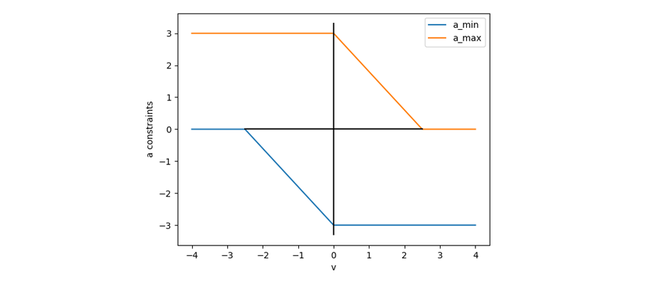
Note the asymmetry between braking and acceleration to illustrate the difference between those two stages. Here’s a simple function used for this model:

def acc_model_simple(v, v1=2.5, a0=3.0, ap=0.0, am=3.0):
    n = len(v)
    a_minus = np.zeros((n,))
    a_plus = np.zeros((n,))
    alpha1 = np.minimum(v[v > 0]/v1, 1)
    alpha2 = np.minimum(-v[v <= 0]/v1, 1)
    a_minus[v > 0] = -(alpha1 * am + (1-alpha1) * a0)
    a_plus[v > 0] = alpha1 * ap + (1-alpha1) * a0
    a_minus[v <= 0] = -(alpha2 * ap + (1-alpha2) * a0)
    a_plus[v <= 0] = alpha2 * am + (1-alpha2) * a0
    return a_minus, a_plus

Here is the solved curve, note the slow acceleration and non-constant boundaries:

unstable optimization

Here is an example with $\lambda=0.8$, the acceleration quickly becomes nonsensical leading to a convergence to a suboptimal curve:

ND motion

Real machines usually have more than one degree of freedom, and acceleration/speed constraints are intertwined in a complex way. Let’s explore the general case and use the tools we discovered in the previous sections.

Problem statement

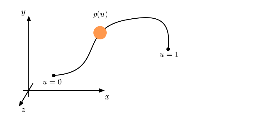
Let’s assume we have a vector motion $\vec{p}(u)$ parametrized by $0 \leq u(t)\leq 1$. By adjusting the rate of the parameter, we can tweak the local speed of the curve. The speed vector of $\vec{p}(u)$ can be expressed from derivatives in $u$ only:

$$\vec{v} = \frac{{\rm d}\vec{p}}{{\rm d}t}=\frac{{\rm d}\vec{p}}{{\rm d}u} \frac{{\rm d}u}{{\rm d}t}:=\frac{{\rm d}\vec{p}}{{\rm d}u} \dot{u}$$

This shows $\dot{u}$ is simply scaling the speed vector. The acceleration vector of $\vec{p}(u)$ is less straightforward:

$$\vec{a} = \frac{{\rm d}^2\vec{p}}{{\rm d}t^2}=\frac{{\rm d}^2\vec{p}}{{\rm d}u^2} \dot{u}^2 + \frac{{\rm d}\vec{p}}{{\rm d}u} \ddot{u}$$

The first term is caused by the curvature of $\vec{p}(u)$, while the second is an acceleration along the curve. As in the previous 1D case, we want to solve $\dot{u}$ and $\ddot{u}$ subject to constraints. The speed constraint is straightforward:

$$\left|\frac{{\rm d}\vec{p}}{{\rm d}t}\right| \leq v_{\rm max}$$

The acceleration constraint, on the other hand, is far from trivial. There is nothing that forces those constraints to be similar in different dimensions. A cartesian machine usually has motors actuating separate axes, which prescribes individual constraints on each axis. Let’s assume this is the case: we can define a cuboid of min/max accelerations around the current acceleration. The shape of this cuboid can also be a function of the vectorial speed:

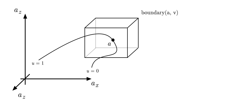
More complex horizon shapes can be introduced in this model to represent different machine configurations. We’ll assume cuboid horizons in the following, leading this form of constraint on the acceleration:

$$a_{{\rm min}, i} \leq \frac{{\rm d}^2 p_i}{{\rm d}t^2} \leq a_{{\rm max}, i}$$

We also want to limit the norm of the jerk per axis:

$$\left|\frac{{\rm d}^3 p_i}{{\rm d}t^3}\right| \leq j_{{\rm max}}$$

Vectorial jerk constraints are also possible, similar to the reasoning on the acceleration.

Phase space representation

As in the 1D case, we choose to solve a reformulation of the problem in a phase space. The equivalent of the position $x$ is now $u$, and the speed $\dot{u}$ takes the role of the speed $v$:

The time is again implicitly defined by:

$$t=\int_0^u \frac{{\rm d} u}{\dot{u}(u)}$$

The problem can be summarized as:

• Minimize $$T=\int_0^1 \frac{{\rm d} u}{\dot{u}(u)}$$

• Subject to:

  • $|\vec{v}(u)| \leq v_{\rm max}~\forall u \in~[0, 1]$
  • $a_{{\rm min}, i} \leq a_i(u) \leq a_{{\rm max}, i}~\forall u \in~[0, 1]$
  • $|j_i(u)| < j_{\rm max}~\forall u \in~[0, 1]$
  • $\dot{u}(0)=\dot{u}(1)=0$
  • $a(0)=a(1)=0$

• With:

  • $\vec{v} = \frac{{\rm d}\vec{p}}{{\rm d}u} \dot{u}$
  • $\vec{a} = \frac{{\rm d}^2 \vec{p}}{{\rm d}u^2} \dot{u}^2 + \frac{{\rm d} \vec{p}}{{\rm d}u} \ddot{u}$

Discrete solver

Let’s work with a discrete version of the parameter $u(k)$ and the parameter speed $\dot{u}(k)$, with $k=0\dots N-1$.

The steps in the solver are adapted directly from the 1D version:

1. Start with a small value for $\dot{u}(k), k \in [1, N-2]$.
2. Evaluate accelerations $a_i(k)$ from $\dot{u}(k)$.
3. Given jerk and acceleration constraints, compute horizons $\ddot{u}_{{\rm min}, i}(k)$ and $\ddot{u}_{{\rm max}, i}(k)$ for each segment.
4. Given $\ddot{u}_{{\rm min}, i}(k)$ and $\ddot{u}_{{\rm max}, i}(k)$ and speed limit, evaluate horizons $\dot{u}_{\rm min}(k)$ and $\dot{u}_{\rm max}(k)$ for each point.
5. Update $\dot{u} \Rightarrow \lambda \dot{u}_{\rm max} + (1-\lambda) \dot{u}$
6. Repeat steps 2-5 until $|\dot{u}_{\rm max} - \dot{u}|_2 < \epsilon$

Step 3 is similar to the 1D case, but there is now a vectorial acceleration constraint:

def constraints_a(p_prime, p_prime2, u, u_dot, jerk_max, a_start=None, a_end=None, show=False):
    n, n_dims = p_prime.shape

    a = np.zeros((n-1, n_dims))

    a_minus = np.zeros((n-1, n_dims))
    a_plus = np.zeros((n-1, n_dims))

    u_mid = 0.5 * (u[:-1] + u[1:])
    u_dot_mid = 0.5 * (u_dot[:-1] + u_dot[1:])
    p_prime_mid = 0.5 * (p_prime[:-1, :] + p_prime[1:, :])
    p_prime2_mid = 0.5 * (p_prime2[:-1, :] + p_prime2[1:, :])
    u_dot_prime = (u_dot[1:] - u_dot[:-1]) / (u[1:] - u[:-1])
    dt = (u[1:] - u[:-1]) / u_dot_mid
    dt_a = (dt[:-1] + dt[1:]) * 0.5

    u_dot2_min_all = -np.inf * np.ones((n - 1, n_dims))
    u_dot2_max_all = np.inf * np.ones((n - 1, n_dims))

    v = np.zeros((n-1, n_dims))
    for i in range(n_dims):
        v[:, i] = p_prime_mid[:, i] * u_dot_mid
        a[:, i] += p_prime2_mid[:, i] * u_dot_mid * u_dot_mid
        a[:, i] += p_prime_mid[:, i] * u_dot_mid * u_dot_prime

        if a_start is None:
            a_minus[0, i] = a_minus_prev[0]
            a_plus[0, i] = a_plus_prev[0]
        else:
            a_minus[0] = a_start[i] - jerk_max * dt_a[0]
            a_plus[0] = a_start[i] + jerk_max * dt_a[0]

        if a_end is None:
            a_minus[-1, i] = a_minus_next[-1]
            a_plus[-1, i] = a_plus_next[-1]
        else:
            a_minus[-1] = a_end[i] - jerk_max * dt_a[-1]
            a_plus[-1] = a_end[i] + jerk_max * dt_a[-1]

        a_plus_next = a[:-1, i] + jerk_max * dt_a
        a_minus_next = a[:-1, i] - jerk_max * dt_a
        a_plus_prev = a[1:, i] + jerk_max * dt_a
        a_minus_prev = a[1:, i] - jerk_max * dt_a

        a_minus[1:-1, i] = np.maximum(a_minus_next[:-1], a_minus_prev[1:])
        a_plus[1:-1, i] = np.minimum(a_plus_next[:-1], a_plus_prev[1:])

        # min and max prescribed by speed
        a_neg_bound, a_pos_bound = a_mp_func(v[:, i])
        a_minus[:, i] = np.minimum(a_minus[:, i], a_pos_bound)
        a_minus[:, i] = np.maximum(a_minus[:, i], a_neg_bound)
        a_plus[:, i] = np.minimum(a_plus[:, i], a_pos_bound)
        a_plus[:, i] = np.maximum(a_plus[:, i], a_neg_bound)

        # acceleration along the curve only
        a_plus_along = a_plus[:, i] - p_prime2_mid[:, i] * u_dot_mid*u_dot_mid
        a_minus_along = a_minus[:, i] - p_prime2_mid[:, i] * u_dot_mid*u_dot_mid

        mask = np.abs(p_prime_mid[:, i]) > 1e-7

        u_dot2_1 = a_plus_along[mask]/p_prime_mid[mask, i]
        u_dot2_2 = a_minus_along[mask]/p_prime_mid[mask, i]
        u_dot2_min_all[mask, i] = np.minimum(u_dot2_1, u_dot2_2)
        u_dot2_max_all[mask, i] = np.maximum(u_dot2_1, u_dot2_2)

    u_dot2_min = np.max(u_dot2_min_all, axis=-1)
    u_dot2_max = np.min(u_dot2_max_all, axis=-1)

    return u_dot2_min, u_dot2_max

Step 4 is more straightforward, as we only wanted to limit the scalar norm of $\vec{v}$. As explained in the 1D scenario, we use an updated $\Delta t$ to improve the precision of the horizon on $\dot{u}(k)$:

def constraints_v(p_prime, u, u_dot, u_dot2_min, u_dot2_max, v_abs_max, v_start=None, v_end=None, show=False):
    n, n_dims = p_prime.shape
    u_dot_min = np.zeros((n,))
    u_dot_max = np.zeros((n,))

    # v = np.zeros((n - 1, n_dims))
    du = u[1:] - u[:-1]
    u_dot_max_next = np.sqrt(np.maximum(u_dot[:-1]**2 + 2 * u_dot2_max * du, 0))
    u_dot_min_next = np.sqrt(np.maximum(u_dot[:-1]**2 + 2 * u_dot2_min * du, 0))
    u_dot_min_prev = np.sqrt(np.maximum(u_dot[1:]**2 - 2 * u_dot2_max * du, 0))
    u_dot_max_prev = np.sqrt(np.maximum(u_dot[1:]**2 - 2 * u_dot2_min * du, 0))

    if v_start is None:
        u_dot_max[0] = u_dot_max_prev[0]
        u_dot_min[0] = u_dot_min_prev[0]
    else:
        # constrain start speed
        u_dot_max[0] = v_start/np.linalg.norm(p_prime[0])
        u_dot_min[0] = u_dot_max[0]

    if v_end is None:
        u_dot_max[-1] = u_dot_max_next[-1]
        u_dot_min[-1] = u_dot_min_next[-1]
    else:
        # constrain start speed
        u_dot_max[-1] = v_end/np.linalg.norm(p_prime[-1])
        u_dot_min[-1] = u_dot_max[-1]

    u_dot_min[1:-1] = np.maximum(u_dot_min_next[:-1], u_dot_min_prev[1:])
    u_dot_max[1:-1] = np.minimum(u_dot_max_next[:-1], u_dot_max_prev[1:])
    u_dot_min = np.minimum(u_dot_min, u_dot_max)

    p_prime_norm = np.linalg.norm(p_prime, axis=-1)
    u_dot_min[:] = np.maximum(u_dot_min, 0)
    u_dot_max[:] = np.minimum(u_dot_max, v_abs_max / p_prime_norm)

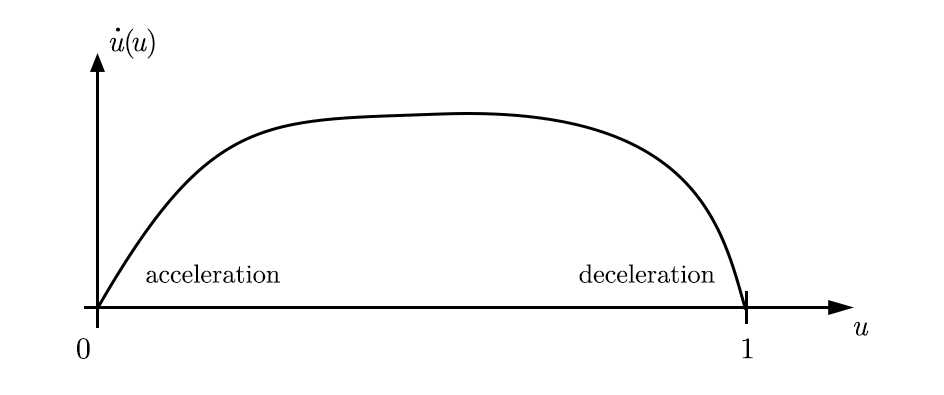
    if show:
        plt.figure()
        plt.plot(u, u_dot, 'k')
        plt.plot(u, u_dot_min, 'b')
        plt.plot(u, u_dot_max, 'r')
        plt.title("u_dot")

    return u_dot_min, u_dot_max

Putting it all together:

# acceleration horizon
u_dot2_min, u_dot2_max = constraints_a(p_prime, p_prime2, u, u_dot, jerk_max)

# speed horizon
u_dot_min, u_dot_max = constraints_v(p_prime, u, u_dot, u_dot2_min, u_dot2_max, v_abs_max)

# update
u_dot = lambd * u_dot_max + (1 - lambd) * u_dot

Results

Bezier spline

Let’s take as a trajectory a bezier spline with handles [0, 0], [2.5, 0], [-0.5, 1], [2, 1] and the regular parametrization $u$:

Here’s a solved $\dot{u}$ curve:

Note the zero-acceleration part in the center due to the curve being almost linear and the speed maximized there. By increasing the jerk constraint, we get a completely different solution:

Here is visualization of the position over time with speed and acceleration vectors displayed on top:

Conclusions

We have shown phase space solvers for both 1D and ND trajectories. While the results are able to find known results in machine control as well as handle dynamic acceleration and jerk within a very general framework. However, the stepwise update rule is very slow, and is an indirect way to handle the constrained optimization problem. Other optimizers should be considered, which can also bring more stability in the results.

Acceleration models more closely inspired by real machines should also be considered.

Finally, the discrete nature of the solution is an issue for using the curve as a solution, which calls for either an interpolation method or a compressed representation. The latter is especially promising for streaming the solution to a machine live.