Consider the damped wave equation

$$\frac{\partial^2 u}{\partial t^2} = v^2 \frac{\partial^2 u}{\partial x^2} + \gamma \frac{\partial}{\partial t}\frac{\partial^2 u}{\partial x^2}\tag{10.52}$$

Take the solution domain to be the interval [0,1]

(a) Use the Galerkin method to find an approximating system of differential equations.

Let's apply the different types of derivatives found in the wave equation:

$$\frac{\partial^2 u}{\partial t^2} = \sum_i a''_i(t) \varphi_i(x)$$$$\frac{\partial^2 u}{\partial x^2} = \sum_i a_i(t) \varphi''_i(x)$$$$\frac{\partial}{\partial t}\frac{\partial^2 u}{\partial x^2} = \sum_i a'_i(t) \varphi''_i(x)$$

We can use these in the Galerkin integral:

$$\int \left[ \frac{\partial^2 u}{\partial t^2} - v^2 \frac{\partial^2 u}{\partial x^2} - \gamma \frac{\partial}{\partial t}\frac{\partial^2 u}{\partial x^2}\right] \varphi_j(x) {\rm d}x = 0$$

Becomes:

$$\sum_i \int \left[ a''_i \varphi_i \varphi_j - v^2 a_i \varphi''_i \varphi_j - \gamma a'_i \varphi''_i \varphi_j \right] {\rm d}x = 0$$

Which can be rewritten as:

$$\sum_i \left[ a''_i <\varphi_i|\varphi_j> - v^2 a_i <\varphi''_i|\varphi_j> - \gamma a'_i <\varphi''_i|\varphi_j> \right] = 0$$

Introducing the notation:

$$<a(x)|b(x)>=\int a(x) b(x) {\rm d}x$$

The system of equation can be summarized as:

$$A.\vec{a}'' + B.\vec{a}' + C.\vec{a} = \vec{0}$$

With:

$$ \begin{cases} A_{ij} = <\varphi_i|\varphi_j>\\ B_{ij} = -\gamma <\varphi''_i|\varphi_j>\\ C_{ij} = -v^2 <\varphi''_i|\varphi_j> = \frac{v^2}{\gamma} B_{ij} \end{cases} $$

Assuming local damped oscillator solutions of the form $\vec{a}(t)=\vec{a}_0 e^{\lambda t}$ with $\lambda \in \mathbb{C}$, the system becomes:

$$A.\vec{a}_0 \lambda^2 + B.\vec{a}_0 \lambda + C.\vec{a}_0 = \vec{0}$$

(b) Evaluate the matrix coefficients for linear hat basis functions, using elements with a fixed size of $h$.

Let's formally define the basis functions:

$$ \varphi_i= \begin{cases} \frac{x-(hi-h)}{h}=\frac{x}{h}-(i-1) & h(i-1)\leq x < hi\\ \frac{(hi+h)-x}{h}=(i+1)-\frac{x}{h} & hi\leq x < h(i+1)\\ 0 & {\rm otherwise} \end{cases} $$

We can plot a $\varphi_i$ and its two neighbors for a step size $h=1$:

A single hat only interacts with its two direct neighbors. Therefore, matrix $A$ only has three active diagonals, and needs to be symmetrical. The two cases are:

$$ \begin{cases} A_{ii} = \int \varphi_i^2 {\rm d}x = 2\int_0^h \left(1-\frac{x}{h}\right)^2 {\rm d}x = \frac{2}{3} h\\ A_{i(i+1)} = \int \varphi_i \varphi_{i+1} {\rm d}x = \int_0^h \left(1- \frac{x}{h}\right) \frac{x}{h} {\rm d}x = \frac{1}{6}h \end{cases} $$

We can also compute $B$ in the same way, but it involves second order derivates, which is definitely an issue with a function with a non-continuous first derivative. We can still give it an attempt by using Dirac impulses:

$$ \varphi'_i = \begin{cases} \frac{1}{h} & h(i-1)\leq x < hi\\ -\frac{1}{h} & hi\leq x < h(i+1)\\ 0 & {\rm otherwise} \end{cases} $$$$ \varphi''_i = \frac{1}{h}\delta \left(x-h(i-1) \right) - \frac{2}{h}\delta \left(x-hi\right) + \frac{1}{h}\delta \left(x-h(i+1)\right) $$

Let's plot the first and derivative, representing a Dirac impulse by its norm:

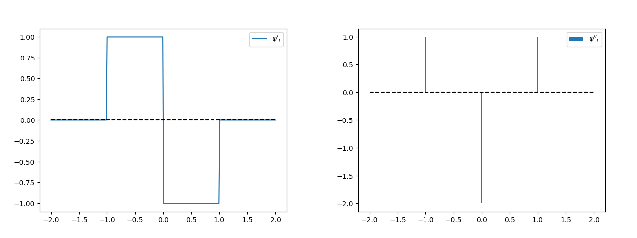
This lets us compute $B$, using the properties of $\delta(x)$:

$$ \begin{cases} B_{ii} = -\gamma \int \varphi''_i \varphi_i {\rm d}x = - \frac{2}{h} \varphi_i(hi) = -\frac{2}{h}\\ B_{i(i+1)} = -\gamma \int \varphi''_i \varphi_{i+1} {\rm d}x = \frac{1}{h} \varphi_{i+1}(h(i+1)) = \frac{1}{h} \end{cases} $$

(c) Now find the matrix coefficients for Hermite polynomial interpolation basis functions, once again using elements with a fixed size of $h$. A symbolic math environment is useful for this problem.

Let's first find the Hermite polynomials. We have to inverse the following:

$$ M= \begin{bmatrix} 1 & 0 & 0 & 0\\ 0 & 1 & 0 & 0\\ 1 & h & h^2 & h^3\\ 0 & 1 & 2 h & 3 h^2\\ \end{bmatrix} $$

Let's use sympy for this:

import sympy
from IPython.display import display, Math

h = sympy.symbols("h", real=True)
M = sympy.Matrix([[1, 0, 0, 0],
                  [0, 1, 0, 0],
                  [1, h, h * h, h * h * h],
                  [0, 1, 2 * h, 3 * h * h]])

display(Math(r"$M^{-1}=$"), M.inv())

$\displaystyle M^{-1}=$

$\displaystyle \left[\begin{matrix}1 & 0 & 0 & 0\\0 & 1 & 0 & 0\\- \frac{3}{h^{2}} & - \frac{2}{h} & \frac{3}{h^{2}} & - \frac{1}{h}\\\frac{2}{h^{3}} & \frac{1}{h^{2}} & - \frac{2}{h^{3}} & \frac{1}{h^{2}}\end{matrix}\right]$

Each column provides the polynomial coefficients for one of the basis splines.

Let's now plot the complete family of splines and their derivatives for a step of $h=1$:

This, whoever, doesn't tell the whole story when using these splines in for the purpose of interpolation. Reflections of the functions are needed to complete the other missing side. Let's plot a centered version of the two kinds of splines, as well as their neighbors. We can also compute the first and second derivatives, note the discontinuity introduced by the reflections:

In those plots, the two functions centered around a point $x_k = hk$ are denoted using $\varphi_{2k}$ and $\varphi_{2k+1}$. Unlike with the hat functions, we now have twice as many basis functions as points $x_k$. This creates confusion with the indices of $A_{ij}$ and $B_{ij}$, which is the reason for introducing a new index $k$.

We see from those plots that for a given $\varphi_i$, there are 6 interactions to consider when computing $A_{ij}$: with itself, with its centered companion, with the two neighboring splines on the left, and the two on the right. We can therefore predict that $A_{ij}$ will have this form:

$$A = \begin{bmatrix} D & E & & & \\ E^{\top} & \ddots & \ddots & & \\ & \ddots & \ddots & \ddots & \\ & & \ddots & \ddots & E \\ & & & E^{\top} & D \\ \end{bmatrix} $$

Where each submatrix is of size $2 \times 2$:

$$D = \begin{bmatrix} <\varphi_0 | \varphi_0> & <\varphi_0 | \varphi_1>\\ <\varphi_1 | \varphi_0> & <\varphi_1 | \varphi_1> \end{bmatrix} $$$$E = \begin{bmatrix} <\varphi_0 | \varphi_2> & <\varphi_0 | \varphi_3>\\ <\varphi_1 | \varphi_2> & <\varphi_1 | \varphi_3> \end{bmatrix} $$

We can compute each integral using sympy:

import sympy

h = sympy.symbols("h", real=True)
x = sympy.symbols("x", real=True)

p1000 = [1, 0, -3/(h*h), 2/(h*h*h)]
p0100 = [0, 1, -2/h, 1/(h*h)]
p0010 = [0, 0, 3/(h*h), -2/(h*h*h)]
p0001 = [0, 0, -1/h, 1/(h*h)]

x_pow = [1, x, x*x, x*x*x]
poly1000 = sum([a*b for a, b in zip(p1000, x_pow)])
poly0100 = sum([a*b for a, b in zip(p0100, x_pow)])
poly0010 = sum([a*b for a, b in zip(p0010, x_pow)])
poly0001 = sum([a*b for a, b in zip(p0001, x_pow)])

D11 = 2*sympy.integrate(poly1000*poly1000, (x, 0, h))
D22 = 2*sympy.integrate(poly0100*poly0100, (x, 0, h))

E11 = sympy.integrate(poly1000*poly0010, (x, 0, h))
E12 = sympy.integrate(poly1000*poly0001, (x, 0, h))
E21 = sympy.integrate(poly0100*poly0010, (x, 0, h))
E22 = sympy.integrate(poly0100*poly0001, (x, 0, h))

display(sympy.Eq(sympy.Symbol(r"D_{11}"), D11))
display(sympy.Eq(sympy.Symbol(r"D_{22}"), D22))

display(sympy.Eq(sympy.Symbol(r"E_{11}"), E11))
display(sympy.Eq(sympy.Symbol(r"E_{12}"), E12))
display(sympy.Eq(sympy.Symbol(r"E_{21}"), E21))
display(sympy.Eq(sympy.Symbol(r"E_{22}"), E22))

$\displaystyle D_{11} = \frac{26 h}{35}$

$\displaystyle D_{22} = \frac{2 h^{3}}{105}$

$\displaystyle E_{11} = \frac{9 h}{70}$

$\displaystyle E_{12} = - \frac{13 h^{2}}{420}$

$\displaystyle E_{21} = \frac{13 h^{2}}{420}$

$\displaystyle E_{22} = - \frac{h^{3}}{140}$

Yielding:

$$D = \begin{bmatrix} \frac{26}{35}h & 0\\ 0 & \frac{2}{105}h^3 \end{bmatrix} $$$$E = \begin{bmatrix} \frac{9}{70}h & -\frac{13}{420}h^2\\ \frac{13}{420}h^2 & -\frac{1}{140}h^3 \end{bmatrix} $$

Following the same reasoning, matrix $B_{ij}$ also has 6 diagonals to consider, and can be written in the form:

$$B = -\gamma \begin{bmatrix} F & G & & & \\ G^{\top} & \ddots & \ddots & & \\ & \ddots & \ddots & \ddots & \\ & & \ddots & \ddots & G \\ & & & G^{\top} & F \\ \end{bmatrix} $$

With:

$$F = \begin{bmatrix} <\varphi''_0 | \varphi_0> & <\varphi''_0 | \varphi_1>\\ <\varphi''_1 | \varphi_0> & <\varphi''_1 | \varphi_1> \end{bmatrix} $$$$G = \begin{bmatrix} <\varphi''_0 | \varphi_2> & <\varphi''_0 | \varphi_3>\\ <\varphi''_1 | \varphi_2> & <\varphi''_1 | \varphi_3> \end{bmatrix} $$

Let's use sympy again to compute the derivatives of the splines, and solving the integrals:

poly1000_deriv = sympy.diff(poly1000, x)
poly0100_deriv = sympy.diff(poly0100, x)
poly0010_deriv = sympy.diff(poly0010, x)
poly0001_deriv = sympy.diff(poly0001, x)

poly1000_deriv2 = sympy.diff(poly1000_deriv, x)
poly0100_deriv2 = sympy.diff(poly0100_deriv, x)
poly0010_deriv2 = sympy.diff(poly0010_deriv, x)
poly0001_deriv2 = sympy.diff(poly0001_deriv, x)

F11 = 2*sympy.integrate(poly1000_deriv2*poly1000, (x, 0, h))
F22 = 2*sympy.integrate(poly0100_deriv2*poly0100, (x, 0, h))

G11 = sympy.integrate(poly1000_deriv2*poly0010, (x, 0, h))
G12 = sympy.integrate(poly1000_deriv2*poly0001, (x, 0, h))
G21 = sympy.integrate(poly0100_deriv2*poly0010, (x, 0, h))
G22 = sympy.integrate(poly0100_deriv2*poly0001, (x, 0, h))

display(sympy.Eq(sympy.Symbol(r"F_{11}"), F11))
display(sympy.Eq(sympy.Symbol(r"F_{22}"), F22))

display(sympy.Eq(sympy.Symbol(r"G_{11}"), G11))
display(sympy.Eq(sympy.Symbol(r"G_{12}"), G12))
display(sympy.Eq(sympy.Symbol(r"G_{21}"), G21))
display(sympy.Eq(sympy.Symbol(r"G_{22}"), G22))

$\displaystyle F_{11} = - \frac{12}{5 h}$

$\displaystyle F_{22} = - \frac{4 h}{15}$

$\displaystyle G_{11} = \frac{6}{5 h}$

$\displaystyle G_{12} = - \frac{1}{10}$

$\displaystyle G_{21} = \frac{1}{10}$

$\displaystyle G_{22} = \frac{h}{30}$

Leading to:

$$F = \begin{bmatrix} -\frac{12}{5h} & 0\\ 0 & -\frac{4h}{15} \end{bmatrix} $$$$G = \begin{bmatrix} \frac{6}{5h} & -\frac{1}{10}\\ \frac{1}{10} & \frac{h}{30} \end{bmatrix} $$