# Robotic Path Planning
Path planning algorithms are used by mobile robots, unmanned aerial vehicles, and autonomous cars in order to identify safe, efficient, collision-free, and least-cost travel paths from an origin to a destination.
## Map representation
Robots are either given, or implicitly build, a mapped representation of their surrounding space. These maps can be saved as:
- a discrete approximations with chunks of equal size (*grid map*) or differing sizes (*topological map*)
- continuous map approximations
Although continuous maps have clear memory advantages, discrete maps are most common in robotic path planning because they map well to graph representations.
[**Occupancy grid maps**](https://en.wikipedia.org/wiki/Occupancy_grid_mapping) discretize a space into square of arbitrary resolution and assigns each square either a binary or probabilistic value of being full or empty. Grid maps can be optimized for memory by storing it as a [k-d tree](https://en.wikipedia.org/wiki/K-d_tree) so that only areas with important boundary information need to be saved at full resolution.
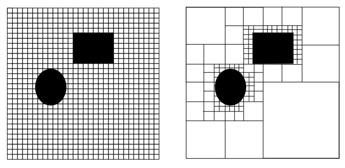
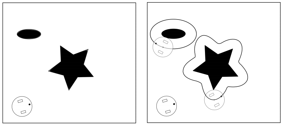
**Configuration space**: To deal with the fact that robots have some physical embodiment which requires space with in the spatial map, configuration space is defined such that the robot is reduced to a point-mass and all obstacles are enlarged by half of the longest extension of the robot.
## General Considerations
### [Goals](https://home.cs.colorado.edu/~mozer/Teaching/Computational%20Modeling%20Prelim/Otte.pdf)
Defines what the path-planner is supposed to achieve, may be a single
objective or a set of objectives.
The most common goal for a path-planning algorithm is finding a path through the C-space from the robot’s current position to another specific goal position.
Examples of other objectives include:
- observing as much of the environment as possible (mapping)
- moving from one location to another while
avoiding other agents (clandestine movement)
- following another agent (surveillance)
- visiting a set of locations while simultaneously attempting to minimize movement (traveling salesman problem).
### [Completeness]
Called **complete** if both:
1. Guaranteed to find a solution in a finite amount of time when a solution exists
2. Reports failure when a
solution does not exist.
**Resolution completeness** means that an algorithm will find a solution in finite time if one exits, but may run forever if a solution does not exist
**Probabilistic completeness** applies to random sampling algorithms. It means that given enough samples, the probability a solution is found approaches 1.
- Does not guarantee the algorithm will find a solution in finite time.
### Geometric Representations
[Geometric Representations](https://webdocs.cs.ualberta.ca/~nathanst/aaai_tut3.pdf) represent obstacles as polygons, i.e. sequences of line
segments (also called constraints)
Find path between two points that does not cross constraints
Advantages:
- Arbitrary polygon obstacles
- Memory efficient
- Topological Abstractions
Disadvantages
- Complex code
- Robustness issues
- Point localization takes more than constant time
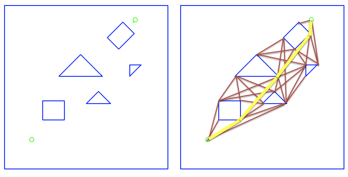
**Visibility graph**
Visibility graph is a graph of inter
visible locations, typically for a set of
points and obstacles in the Euclidean
plane.
Each node in the graph represents a
point location, and each edge represents
a visible connection between them
That is, if the line segment connecting
two locations does not pass through any
obstacle, an edge is drawn between them
in the graph.
Then uses [A\*](https://www.cs.columbia.edu/~allen/F19/NOTES/lozanogrown.pdf) to search for shortest paath via visible vertices.
Path is provably optimal, however, adding and changing world can be expensive as graph can be dense.
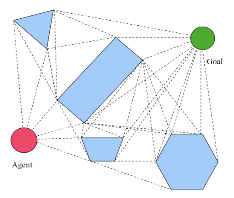
**Free Space Decomposition**
Decompose empty areas into simple convex shapes (e.g. triangles, trapezoids)
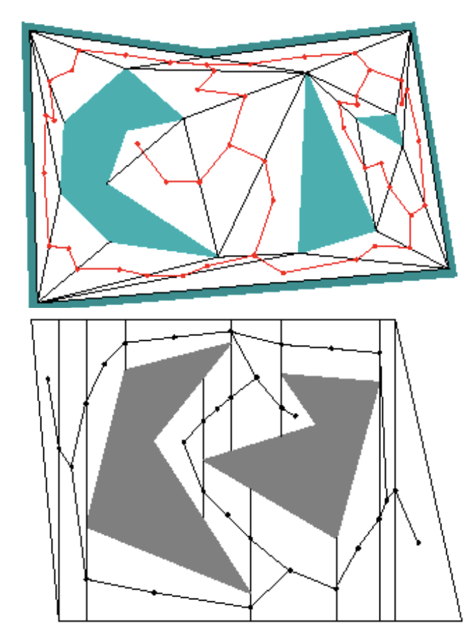
- Create waypoint graph by placing
nodes on unconstrained edges
and in the face interior, if needed
- Connect nodes according to
direct reachability
- Find path from A to B:
1. Locate faces in which A, B
reside
2. Connect A, B to all face nodes
3. Run A*, smooth path
## Tree search algorithms
Once a space is represented as a graph, there are classic shortest-path graph algorithms that can guarantee the shortest path is found, if given unlimited computation time and resources.
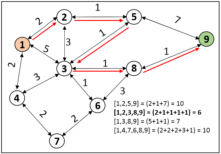
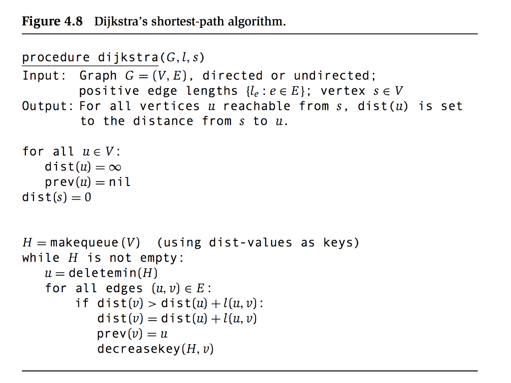
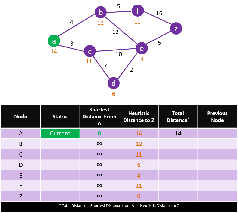
### Dijkstra's algorithm [(1959)](http://www-m3.ma.tum.de/foswiki/pub/MN0506/WebHome/dijkstra.pdf)
Dijsktra's algorithm creates a set of "visited" and "unvisited" nodes, with the initial starting node at a distance of 0, and all other node's set to infinity.
Distances are updated as each neighbor is visited. If the distance is less than the previous distance value, the value is updated.
The algorithm continues until all nodes have been moved from "unvisited" to "visited". [Graph example](https://antonhaugen.medium.com/dijkstras-shortest-path-algorithm-cb8d0a7ae642) below.
### A* [(1968)](https://ieeexplore.ieee.org/document/4082128)
[A\*](https://en.wikipedia.org/wiki/A*_search_algorithm) is another path-finding algorithm that extends Dijkstra's algorithm by adding heuristics to stop certain unnecessary nodes from being searched. This is done by weighting the cost values of each node distance by their euclidean distance from the desired endpoint. Therefore, only paths that are headed generally in the correct direction will be evaluated.
A* is defined as: $f(n) = g(n) + h(n)$ where $g(n)$ is the actual cost from node n to the initial node, and $h(n)$ is the cost of the optimal path from the target node n.
### D* [(1994)](https://citeseerx.ist.psu.edu/viewdoc/summary?doi=10.1.1.15.3683)
[D\*](https://en.wikipedia.org/wiki/D*) is an incremental search algorithm, meaning that it uses information from previous algorithm searches to speed up exploration of the space. D\* generates a collision-free path amidst moving obstacles. D* is an informed incremental search algorithm that repairs the cost map partially and the previously calculated cost map.
## Sampling-based planning
**Complete** versus **resolution complete** algorithms (only as complete as the state-space is, so discretization plays a large role).
Sampling-based planners are **probabilistic complete**, meaning they create possible paths by randomly adding points to a tree until the best solution is found, time expires, or a certain number of points have been chosen.
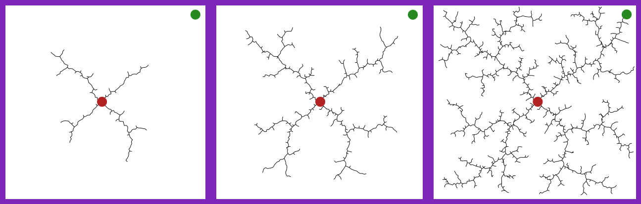
### Rapidly-exploring random trees (RRT) [(1998)](http://msl.cs.uiuc.edu/~lavalle/papers/Lav98c.pdf)
[RRT](https://en.wikipedia.org/wiki/Rapidly-exploring_random_tree) quickly searches a space by randomly expanding a a space-filling tree until the desired target point is found.
The basic algorithm is as follows, for some starting point, *start*, and a ending goal, *goal*
```
tree = init(x, start)
while elapsed_time < t and no_goal(goal):
new_point = stateToExpandFrom(tree)
new_segment = createPathToTree(new_point)
if chooseToAdd(new_Segment):
tree = insert(tree, new_segment)
return tree
```
- **stateToExpandFrom()**: finds the next point to add. This can be completely random search over the state space or can be informed by preferences around nodes with fewer out-degrees (i.e. less connections)
- **createpathToTree()**: this can use the classical shortest-distance graph algorithm for mapping a points to the tree, but that does necessarily choose the overall shortest path. (**RRT\*** is an extension of RRT which connects the point in a way that minimizes the overall path length - this is easiest to do when starting from the goal instead of the starting point.)
- **chooseToAdd()**: needs to check for collisions which can be the most computationally expensive part, especially if the robot can run into itself. There are tricks for "lazy collision evaluation", which only checks for collisions at suitable paths, and if a collision occurs then just that bad segment is deleted, while the rest of the path remains.
## Machine Learning path planning
Machine learning methods are the latest development for determining robotic path planning. Reinforcement learning using **Markov Decision Processes** or deep neural networks can allow robots to modify their policy as it receives feedback on its environment. Classical **Q-learning** algorithms provide a model free learning environment.
- Great overview of Machine Learning approaches to path planning [(Otte 2009)](https://home.cs.colorado.edu/~mozer/Teaching/Computational%20Modeling%20Prelim/Otte.pdf)
- Supervised machine learning for improved rover navigation, using Approximate Clearance Evaluation (ACE) algorithm to evaluation whether the most highly ranked paths are safe. [Here](https://ieeexplore.ieee.org/stamp/stamp.jsp?arnumber=9438337), they trained a model to predict ACE values based on heightmap data (learned heuristic). 2 heuristics were found that produce cost estimates that more effectively rank the candidate paths before ACE evalution.
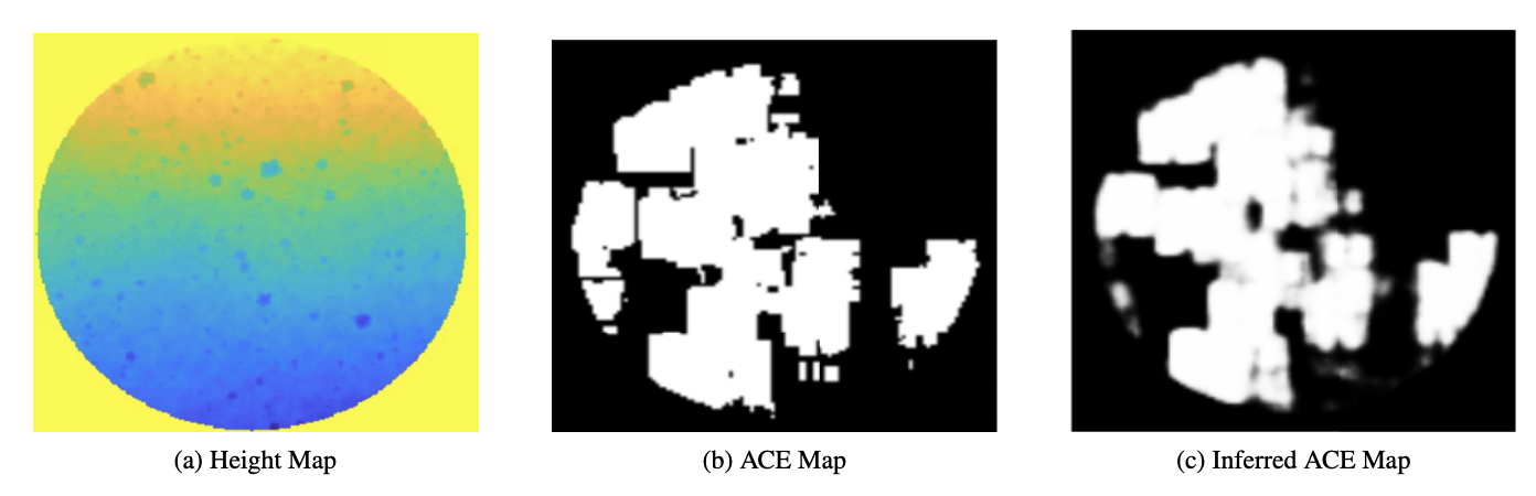
An example of a Learned Heuristic. Sets of terrain heightmaps (a) and maps generated by the ACE algorithm
(b) were used to train a neural network to generate an inferred ACE probability map (c).