(click for larger PDF, 340 KB)
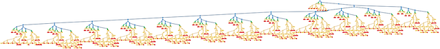
How do you quickly evaluate strings of math/logic?
The code distinguishes between three types of nodes:
X - 0.3atan(Y/X)3.14159 / 2X < 0.3atan(Y/X) < Y3.14159 >= (X-Y)(X < 0.3) && (X > 0.1)(atan(Y/X) < Y) || (X > Y)!(3.14159 >= (X-Y))These nodes are organized in a hierarchical tree: numerical nodes at the bottom, logical nodes
at the top, and transition nodes in between. The gear is visualized below.
(click for larger PDF, 340 KB)
To optimize evalution, these expressions are evaluated over intervals in the plane. Instead of solving at each point, we solve for a square or rectangular region. The result on an interval can be true, false, or ambiguous (e.g. X < 0.5 with 0 < X < 1).
The solver uses quadtrees to take advantage of interval arithmetic. If a region is declared true
or false, then that entire region is colored or white. If a region is ambiguous, then it is subdivided
into four small regions; the process then repeats.

If a logical expression is unambiguous for a region on the plane, then it will remain unambiguous if we subdivide that region. Therefore, it is possible to skip entire branches of the expression; the number of branches skipped increases as the solver recurses into the image. When we pop out of a recursion level, it is necessary to forget the most recent logic-level cache result, since it may no longer be applicable.
The cache is implemented as a list of tribool values. It is used as a reference if the top value is true or false; otherwise, the solver evaluates the logical branch.
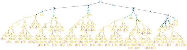
The same expressions - atan2(Y, X), for example - tend to show
up many times in these math strings. The parser checks each node against a list of all known atoms
before pushing it to the output stack. If it matches, then its tree is redirected to point at the
existing identical tree. This turns the tree into a graph, where a node could be referred to by
multiple parents. Each node stores a reference count; nodes are only deleted when their last reference
disappears.
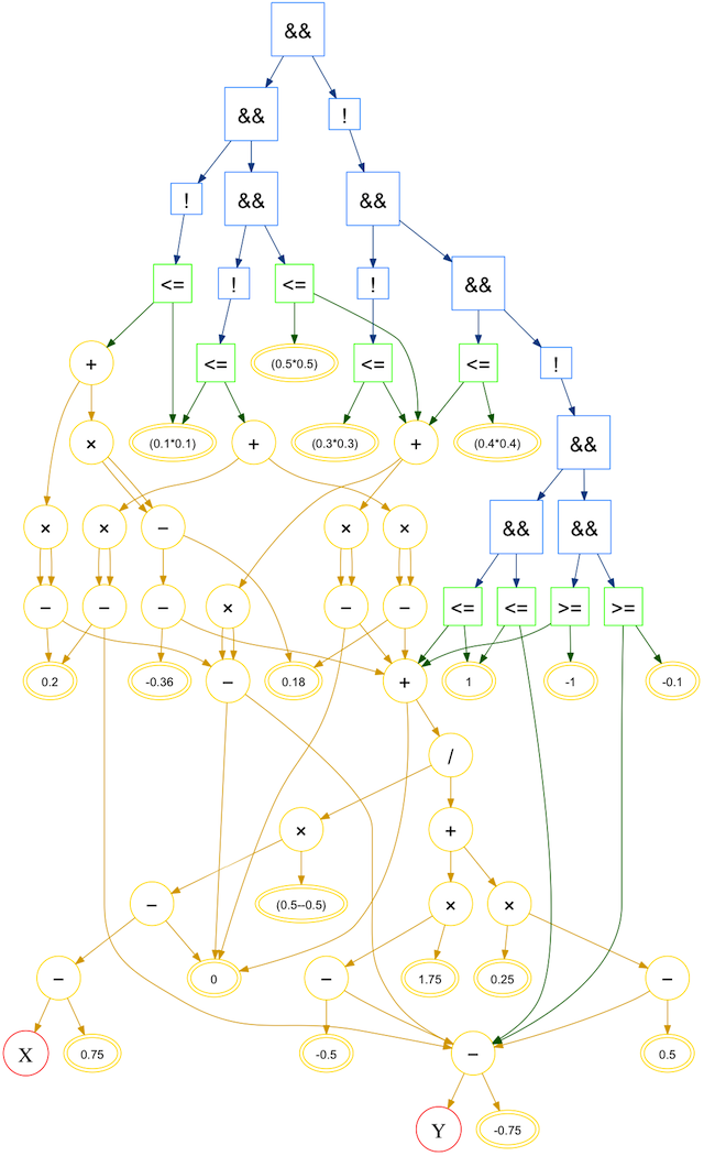
Alien math string without and with node combination:
With this graph structure, it is most efficient to evaluate each node only once. This is handled by an evaluation cache and a variable indicating if the cache is valid. It is inefficient to recurse through the entire tree to reset the cache valid variable. Instead, the solver uses a global cache parity variable. An individual node's cache is valid if its local parity is equal to the global parity, which toggles after each evaluation.
The combination of logical caching and evaluation caching has a few unexpected kinks; for example, branches that are skipped due to logical caching may end up with their evaluation cache in an incorrect parity. For that reason, it is necessary to reset the evaluation cache for all nodes when popping out of a recursion level.
Numerical operations on constants do not change. If a numerical operation has constant arguments, then it is flagged as constant, precomputed, and never computed again.
These comparisons were done timing only the evaluation stage. I ignored parse time for
my program, compile time for math_png, and png write time
for both programs.
| Source | math_png time(seconds) |
Run time (seconds) [optimizations are cumulative] |
|||||
|---|---|---|---|---|---|---|---|
| File | Resolution | None | Quadtree | Logic caching | Node combination | Constant caching | |
| alien | 100 | 0.52 | 42.8 | 2.4 | 0.32 | 0.18 | 0.15 |
| 250 | 3.3 | Long | 15.1 | 2.1 | 1.28 | 1.13 | |
| gear | 100 | 0.76 | Long | 13.1 | 1.19 | 0.65 | 0.52 |
| 250 | 4.8 | Too Long | 81.0 | 6.6 | 3.3 | 2.4 | |
I extended the solver with multithreading. The program is hardcoded to spawn a certain number of threads. Before each recursion, the solver checks to see if the number of threads is less than this maximum. If so, then it clones the expression tree (to prevent in-fighting over the caches) and passes it to a new thread. As threads finish, their parent culls them; once all have returned, the parent process returns.
Early attempts produced hilarious numbers in the activity monitor:

Below are result on render times with multithreading, comparing against
the standard math_png.
| Source | math_png time(seconds) |
Run time (seconds) with varying numbers of threads |
|||||
|---|---|---|---|---|---|---|---|
| File | Resolution | 1 | 2 | 4 | 8 | 16 | |
| alien | 100 | 0.52 | 0.18 | 0.14 | 0.06 | 0.06 | 0.05 |
| 250 | 3.3 | 1.18 | 0.94 | 0.35 | 0.29 | 0.28 | |
| gear | 100 | 0.76 | 0.58 | 0.45 | 0.32 | 0.20 | 0.18 |
| 250 | 4.8 | 2.7 | 2.1 | 1.46 | 0.73 | 0.61 | |
I also extended the system so that it visualizes which parts of the image were computed by which thread. Each thread is assigned a bright color when it is created; it colors all the parts of the image that it computes in its color.

I extended the system to recognize color embedded in 24-bit numerical values: the bottom 8 bits are the red channel, middle 8 are blue, and top 8 are green.
This is a different mode of operation for the solver. Instead of outputing a boolean value at the top level, it outputs an interval.
If the interval is a single, unambiguous value, then we know that is the desired color.
On the other hand, if the result is still a region or contains
NaNs, then the solver recurses further.
When handling PCBs, the parser became the slowest step by orders of magnitude. This was due to two bottlenecks:
The first bottleneck was resolved by switching from boost::regex
to simple C-string based tokenizing. I also switched from a full-string tokenizer to a
just-in-time tokenizer to make things a bit cleaner.
The second bottleneck was solved by pre-sorting nodes into bins based on their operation type. If the parser is looking for duplicates of an addition nodes, it only compares against other addition nodes (rather than against every node in the system).
These improvements make the full-system run time (including parsing and png output) faster
than the existing math_png across a variety of resolutions.
| Source | math_png time(seconds) |
New solver time (seconds) |
Speed-up | |
|---|---|---|---|---|
| File | Resolution | |||
| alien | 10 | 0.213 | 0.03 | 7.1x |
| 20 | 0.246 | 0.046 | 5.3x | |
| 50 | 0.455 | 0.143 | 3.2x | |
| 100 | 1.183 | 0.507 | 2.3x | |
| gear | 10 | 0.267 | 0.033 | 8x |
| 20 | 0.295 | 0.061 | 4.8x | |
| 50 | 0.496 | 0.105 | 4.7x | |
| 100 | 1.200 | 0.271 | 4.4x | |
| hello.ISP.44 | 10 | 1.570 | 1.053 | 1.5x |
| 20 | 2.146 | 1.380 | 1.6x | |
| 50 | 6.283 | 2.109 | 3x | |
| 100 | 19.15 | 3.844 | 5x | |
|
fab boombox case (11 pieces) |
20 | 15.603 | 3.795 | 4x |
Before handing off part of the job to a new thread, the solver needs to clone the math tree. Otherwise, the two threads will fight over the caches (this leads to segfaults and plagues of locust).
Previous versions of the solver cloned the entire math tree. However, with logical-level caching, we can guarantee that certain branches will never be evaluated - so why waste resources cloning them?
I modified the clone function to only clone branches that are not already cached. This didn't have much effect on the gear or alien, but it had a significant impact on pcb evaluation speed.
| Source | Without pruning (seconds) |
With pruning (seconds) |
|
|---|---|---|---|
| File | Resolution | ||
| hello.ftdi.44 | 10 | 0.52 | 0.35 |
| 20 | 0.82 | 0.73 | |
| 50 | 1.03 | 0.72 | |
| hello.ISP.44 | 10 | 1.26 | 0.71 |
| 20 | 1.46 | 0.80 | |
| 50 | 2.14 | 1.26 | |
| hello.arduino.168 | 10 | 2.52 | 1.46 |
| 20 | 2.82 | 1.74 | |
| 50 | 3.74 | 2.42 | |
I extended the solver to handle three-dimensional regions using octrees. Each volume is divided into eight sub-regions, which are solved with the same recursive strategy as earlier.
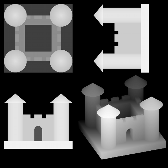
It also generates modern art:

When generating height maps, the solver uses techniques to minimize the number of points that it has to calculate. When subdividing, it operates on regions with high z values first. Moreover, it checks each region to make sure that it isn't completely occluded before solving. Since the image is initialized to all black, this is an easy test - if all of the points x, y in the region are lighter than the corresponding color of the region, then we can skip it.
In comparison to the old version of
math_png (i.e. the version plugs the math string into a c template, compiles,
and runs) we see a significant improvement.
All of the tests below were run at a resolution of 10 pixels/mm, with varying numbers of z slices.
| Source | Old solver (seconds) |
New solver (seconds) |
|
|---|---|---|---|
| File | z slices | ||
| Castle (z view) | 10 | 0.41 | 0.12 |
| 20 | 0.61 | 0.13 | |
| 50 | 1.2 | 0.17 | |
| 100 | 2.1 | 0.3 | |
| Castle (quad view) | 10 | 3.1 | 0.7 |
| 20 | 5.8 | 1.0 | |
| 100 | 14.0 | 1.9 | |
| 50 | 27.4 | 3.7 | |
| brick | 10 | 0.22 | 0.03 |
| 20 | 0.23 | 0.04 | |
| 50 | 0.28 | 0.08 | |
| 100 | 0.35 | 0.08 | |
Previously, colors were implemented as integer bitfields. In the new solver's hierarchy,
they existed as numerical nodes, operating on intervals of doubles.
I changed the solver's implementation to make colors a distinct type of node in the tree. Everything still looks and acts the same (except for really pathological cases, and I have no qualms about breaking those), but the solver is being a bit smarter.
It creates a colored node whenever we multiply a boolean by a numerical value. Further logical operations on the colored node (and/or/not) modify the color bitfield.
Knowing which nodes are colored regions allows for more intuitive behavior. Booleans and numerical values are automatically promoted to colored regions when combined with a pre-existing colored region. For example, combining a colored region with a boolean will auto-promote the boolean to pure white, rather than leaving it as a single bit of red.
The (pretty much converged) solver was rewritten to take advantage of a new evaluation paradigm: solving the trees from the bottom up rather than from the top down.
Instead of using recursion and recursing down the tree branches, the new solver sorts nodes by weight (e.g. constants and variables have weight 0, everything else has the largest children's weight plus one). It then solves each weight category, starting from 0 up until the top of the tree.
When a node is solved, it stores the result in a local variable. When it needs a child's result, it queries that child's result variable. Because of the evaluation order, a child's variable is guaranteed to be set by the time a parent needs to look at it.
Since these variables are persistant, a node is automatically cached if we no longer evaluate it. This is implemented by swapping a node to the end of the list, then decreasing a counter that keeps track of "active nodes".
When a tree is cloned (to be handed off to a new thread), only the active nodes are cloned. The other nodes stay where they are, cached in place, and may be pointed to by the cloned nodes.
The results of this new solver show a strong improvement for complex math strings.
| Source | Before rewrite (seconds) |
After rewrite (seconds) |
|
|---|---|---|---|
| File | Resolution | ||
| hello.ftdi.44 | 10 | 0.343 | 0.195 |
| 20 | 0.397 | 0.223 | |
| 50 | 0.622 | 0.367 | |
| hello.ISP.44 | 10 | 0.698 | 0.328 |
| 20 | 0.705 | 0.388 | |
| 50 | 1.045 | 0.796 | |
| hello.arduino.168 | 10 | 1.208 | 0.611 |
| 20 | 1.338 | 0.691 | |
| 50 | 1.870 | 1.237 | |
The rewritten solver is also faster for 3d shapes. All of the tests below were run at 10 pixel/mm resolution and varying numbers of z slides.
| Source | Before rewrite (seconds) |
After rewrite (seconds) |
|
|---|---|---|---|
| File | z slices | ||
| Castle (z view) | 10 | 0.103 | 0.092 |
| 20 | 0.107 | 0.098 | |
| 50 | 0.168 | 0.139 | |
| 100 | 0.287 | 0.182 | |
| Castle (quad view) | 10 | 0.691 | 0.527 |
| 20 | 1.009 | 0.676 | |
| 50 | 2.078 | 1.066 | |
| 100 | 4.083 | 1.676 | |
| brick | 10 | 0.032 | 0.027 |
| 20 | 0.047 | 0.035 | |
| 20 | 0.099 | 0.045 | |
| 100 | 0.091 | 0.056 | |