Moritz Kassner
Jump ahead scroll down
Please note: There are 8 or so Vimeo movies embedded. If they don't show please reload.
Environments: Make a ball bounceOrdinary Differential Equations
Environments: Tests with OpenGL
Finite Difference: Ordinary Differential Equations
Finite Difference: Partial Differential Equations
Random Systems
Cellular Automata
Cellular Automata in Numpy
Data Fitting
Transforms
Search
Ctypes in Python
Final Project
Getting Started: Environments
Make a Ball bounce with Python, OpenGL and Pygame. I knew python but I have never done anything with OpenGL or Pygame.
I also did a version with Python that animated balls through RhinoScript and a version in Processing
Code:
Processing CodePython, Pygame and PyOpenGl
Python RhinoScript
Experiments wit OpenGl
The problem with OpenGl legacy calls like Triangle or TriangleStrip is that you waste all your CPU on making slow Python calls. Instead you can be smarter and use Vertex Buffer Objects to dynamically link Python Object with Memory on the Graphics Card. This way you set up your Geometry once and from then on just tell OpenGl you use the referenced Vertex and Texture Objects. Unfortunatly I have not pushed this far enough to make it useful - I will continue to work on it in the future.
Code:
Python VBO codeOrdinary Differential Equations
Having last been exposed to real math in Hi-school this one was tough. I first had to get used to complex numbers and their handiness in describing occilantions- Most experiments here I did with Mathematica.
homework 1 a and b.pdfhomework 1 c 2.pdf
Laplace Transform.pdf
Q-Factor.pdf
Finite Difference ODEs
So much I did not know and very eye-opening, in collaboration with Ari Kardassis
Comparing Euler Step with Adaptive RungaKutta on a undampend, undriven oscilation. Note how poorly Euler Step () performs, even though its stepsize is smaller, it is numerically unstable and quickly explodes. Not so the adaptive Runga Kutta stepper, note how it increases its inital (smaller that necessary) step size, still meats a specified error threshold and stays numerically stable.
If the system in not as nicely behaved as the one before, like this pendulum on a oscillating base, even the tiniest disturbance will eventually show dramatic consequences, these systems are inherently chaotic. Even the sophisticated Adaptive-Runga-Kutta solver quickly diverges. Here two identical runs differ by an offset of 0.000000001 in their initial conditions.
This is such a chaotic pendulum simulated with the Adaptive-Runga-Kutta stepper and rendered in OpenGL. Note that the animation is not a a consistent frame rate. This is not because the step sizes differ (thats what the adaptive stand for - and Ari and I compensate for it) - is because my CPU is to weak to do screen capture and run the program at the same time.
Code:
Python Vector Class by Ari Kardassis - very usefullThe acutal solver code
Main, Setup, OpenGl and Render Code
Finite Difference PDEs
Numerically solving Partial Differential Equations, in collaboration with Ari Kardassis
Solving a 1D string over time and space. Space on the x-axis (the string), time on the y-axis and value in z. Here you can see that information has to travel faster than the process (as it does in (1)) - otherwise you will run into numerical errors (2) if you increase the time step even more it eventually leads to a numerical explosion (3). Looking at the code you will see the implicit and the explicit method for solving this problem.
Solving Fields - in this case the Heat Equation. Here with ADI (Alternating Direction Implicit Method) were the progression of the field in time is solved half way implicitly on rows by inverting a Tri-Diagonal Matrix and explicitly on the colons.This is repeated alternating the rows and colons every step. It allows for bigger steps sizes and is numerically stable.
Successive Over relaxation (SOR) is good if you only care about the end result.The wave you see it the propagation of the the information though the lattice - its direction depends on how the lattice is processed by the solver. See code for more details. Interesting here is that you can choose how much you want to overcorrect. This is a knob who's optimal value depends on the lattice size and the problem to be solved, to little slows down the process, too much will make the SOR diverge numerically. Knowing how to hit the sweet-spot is non-trivial and just above it there are some nice artifacts to be observed. (see video)
Code:
The main FunctionNote the controls: Mouse to orbit, Space to toggle render mode, also play with 1,2,n c e and use a to toggle between SOR adn ADI
The Plane ClassThe Solvers
Cellular Automata
Python Long word implementation. Runs super fast as song as you don't look at the data! It works on a hexagonal grid and I did not un-skew the lattice. Pygames Nd_array to PIL is used to Push the pixels to the Screen.
Code:
CA codeGrid class
Cellular Automata with NumPy
I looked at the code again and made a version using NumPys roll function which can be used as a cyclical bit-shift. I really learned to appreciate NumPys array functions - they can be quite powerful!. I think the code is very clean. But again displaying it is very costly.
Code:
CA NumPy CodeScipy, Numpy, and Matplotlib for MacOS 10.5+
If you want to install this bundle AND you are using the python version that comes with MacOS, I highly recommend Scipy-Superpack.
C-Types in Python
I really like python - its a joy to write with when you make small programs (which is all I do most of the time).
But when Peter-Schmidt-Nielson shows his Cellular Automata running with C-Speed (299 792 458m/s = it feels about 1000 times faster than python)
I cant help myself to notice just how slow python is. Also of course how well Peter writes code.
C-types is very nice. Heavily borrowing from this tutorial and its comments I have made a C-types tutorial that is confirmed to run on Mac os 10.6 with native python and the version of gcc that comes with X-code.
1) write your c function and save in folder all your code will be in as FILENAME.c
2) open Terminal: cd to the working dir
3) type: gcc -shared -fPIC FILENAME.c -o FILENAME.so
4) create your py file and add at least the following:
from ctypes import *
NAMEOFYOURC-TYPES_LIB = CDLL("FILENAME.so")
done!
you now have access to your c functions within python: NAMEOFYOURC-TYPES_LIB.multipy(10,20)
of course the tricky part is overcoming the differences of Typing in C and Python - also very usefull is the use of Pointers.
Check out the examples here:
Simple (from fsckd.com):
libtest.c
libtest.py
with Pointer and Typing (by: frikker@gmail.com):
pointerlib.c
pointerlib.py
Data Fitting
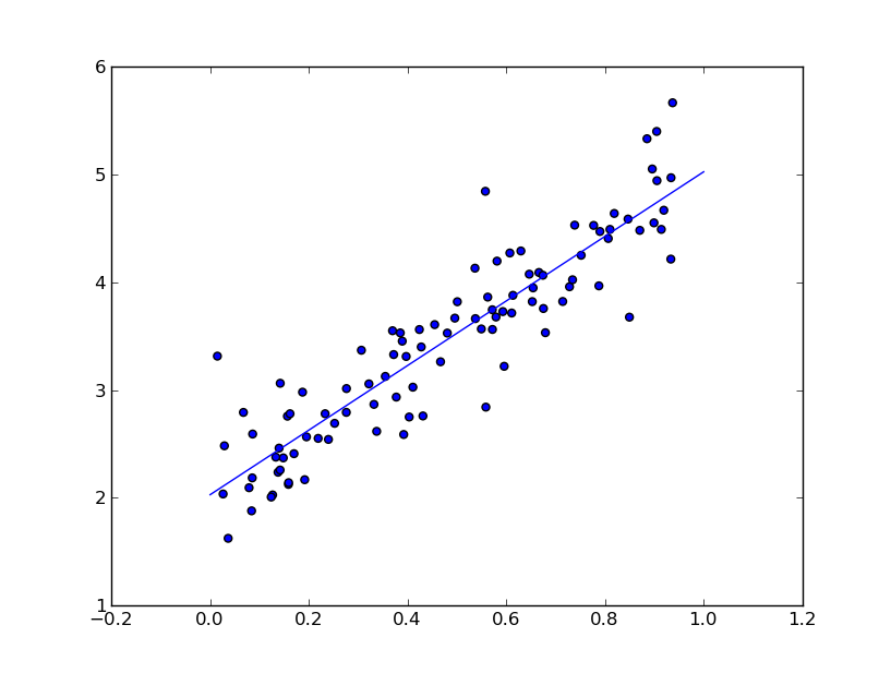
Fitting Data using least squares fit and others, more in the code... Also check out the final Project it has more elaborate SVD code.
Code:
Data fitting codeTransforms
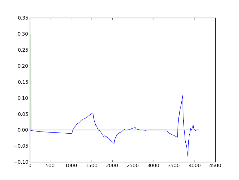
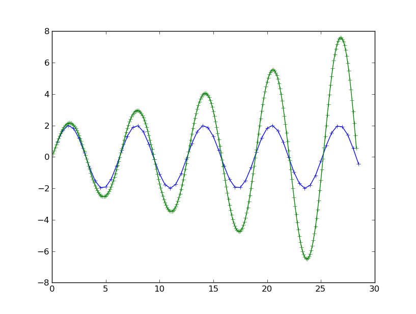
Transforms. Wavelet transform from Wavelet (green) to signal (blue).I actually implemented it with Matrices which is very slow. For PCA - its in the Code.
Code:
Wavelet Transform codeCovariance code
Warning, incomplete...
Search
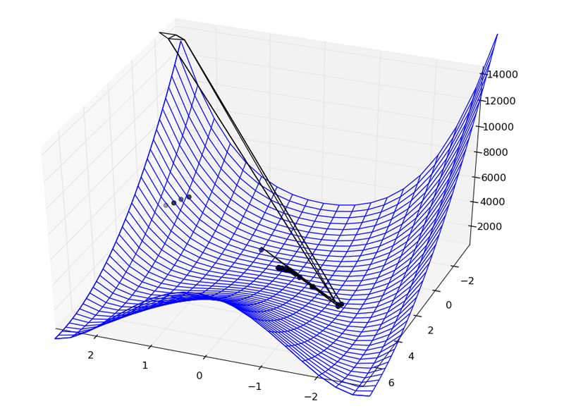
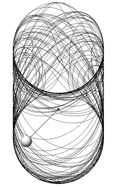
Simplex - a multidimensional search algorithm in under 40 lines of code - very nice. The lines are the trace of the simplex , the dots are the vertex projection to the xy-plane. The function is called the Rosenbrock function its minimum is at 1,1
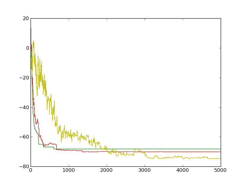
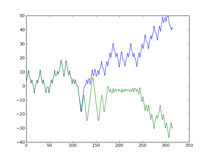
Searching for the lowest energy configuration using simulated annealing, with red green (10 times slower) and gold (100 times slower) having different cooling rates.
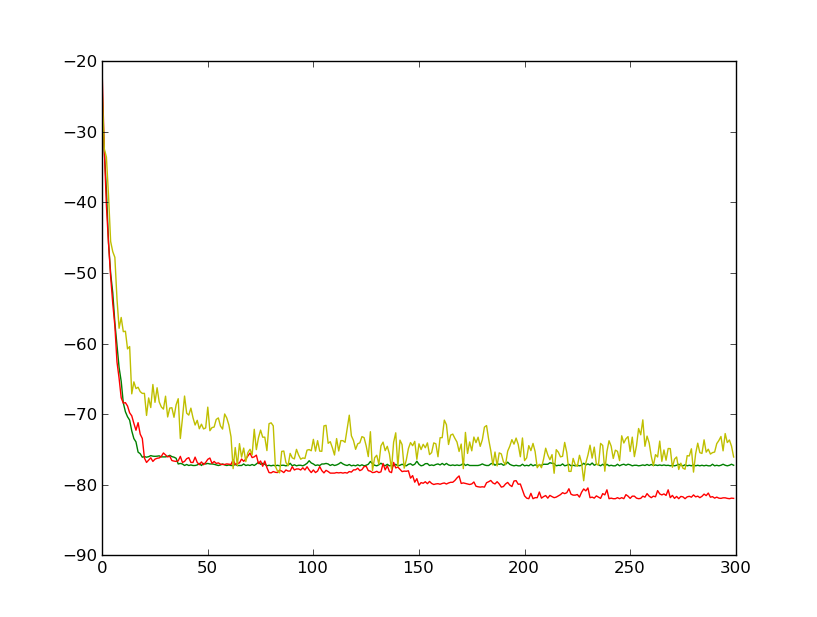
Here a Genetic Algorithm is used to search for the lowest energy configuration. Again with different parameters this time it sets how much performance weights into the reproduction selection.
Code:
Simplex CodeSimulated Annealing and GA-Search