Final Project - Optimization of Structures
This page focuses on my semester project for MAS.864. I extended the finite element method covered in class to model a frame structure comprised of multiple beams. The resulting program executes quickly, and can animate the variation of loading of a reasonably complex structure in "real time". Once this stage was complete, I took a very simple structure consisting of two beams connected at a single point, and began to implement and apply optimization algorithms.
Work log - I maintained a journal-style record of my work on the final project during the semester. Click here to view it
1. Background
There is a long and rich history of using optimization techniques in structural design problems. Perhaps the earliest example is the analytical work of Michell in 1901. The pioneering work of Heyman in the 1970s focused primarily on optimizing the size of members for a fixed topology and geometry, formulated as Linear Programs. Most of the work around that time focused on truss structures, most likely due to their relatively straightforward mathematical expression. Later efforts addressed the problem of geometry optimization, where the nodes of the structure are allowed to move around. The problem of topology optimization, where the connectivity of structural elements is decided by an algorithm, has been most successfully addressed by the SIMP (Solid Isotropic Material with Penalization) method, although a wide variety of other methods have been developed and applied. Topology optimization of structures is still an active research area. Recent years have seen a virtually exhaustive application of search techniques such as genetic algorithms, simulated annealing and particle swarm methods to structural design problems, with multi-objective and multi-physics approaches becoming more common. The problem of simultaneous geometry and sizing optimization of frame structures has been fairly well studied, and will constitute the initial focus of this project.
2. Modeling of Frame Structures
This part of the project focused on modeling two-dimensional frame structures using the finite element method with second-order (Hermite polynomial basis functions) elements. Some of the difficulties in scaling up from the simple beam modeling we covered in class include the fact that the connectivity of the elements is not as straightforward, the orientations of the elements are not all the same, and the construction of the global stiffness matrix from the element stiffness matrices is a little more difficult (because of varying element connectivity and element orientations). A more detailed look at some of these issues is given on this page. The source code for modeling and analyzing the frame structure is in this Python class. I have defined a structure for the input data, and two examples of generating and analyzing structures are given in this Python code. It generates the simple beam structure used in the first optimization steps, and then a more complex one. All the numerical work is done by the numpy library, and pygame is used for visualization. The video below shows the pygame animation of the second structure. Vertical loading on the bottom right node is varied cyclically. This is not a simulation of the structure's dynamic behavior - it is a series of static analyses shown sequentially
3. Unconstrained Minimization of a Simple Structure
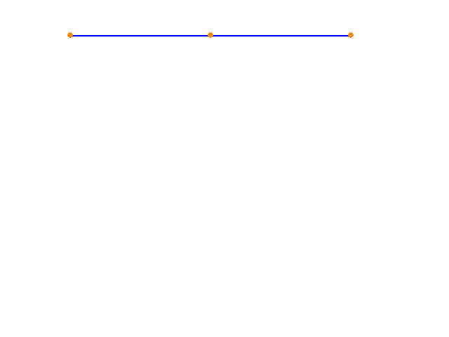
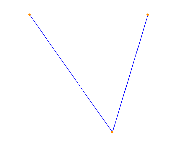
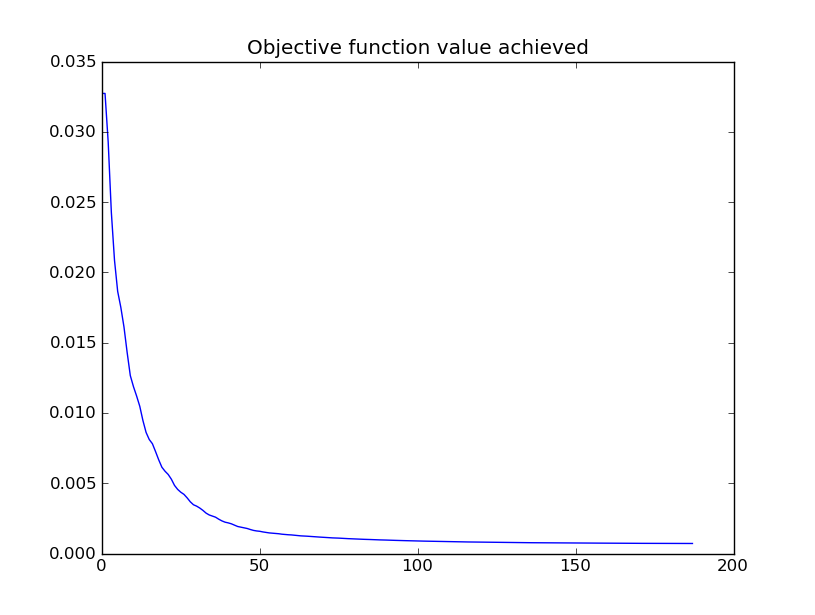
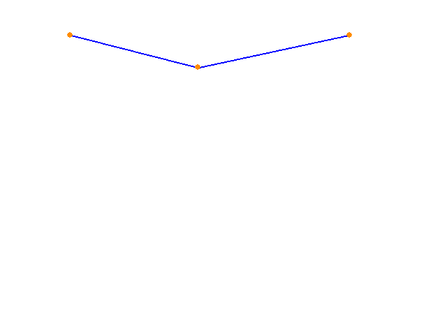
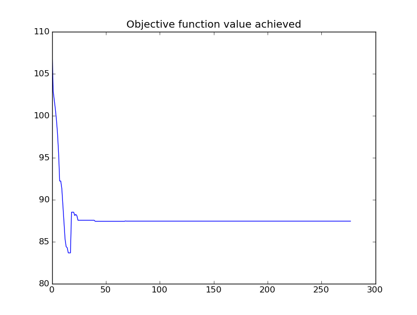
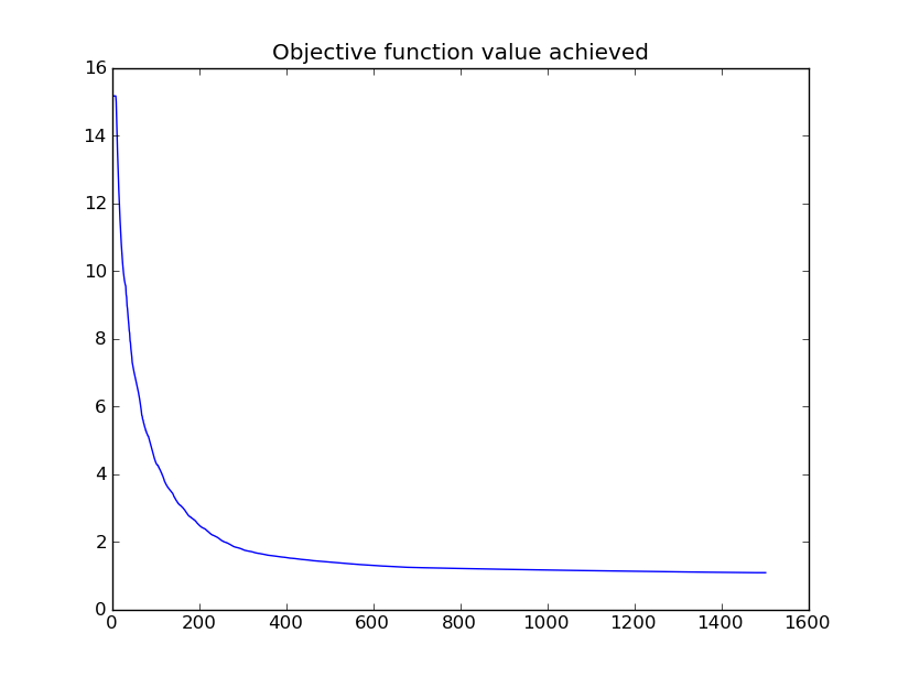
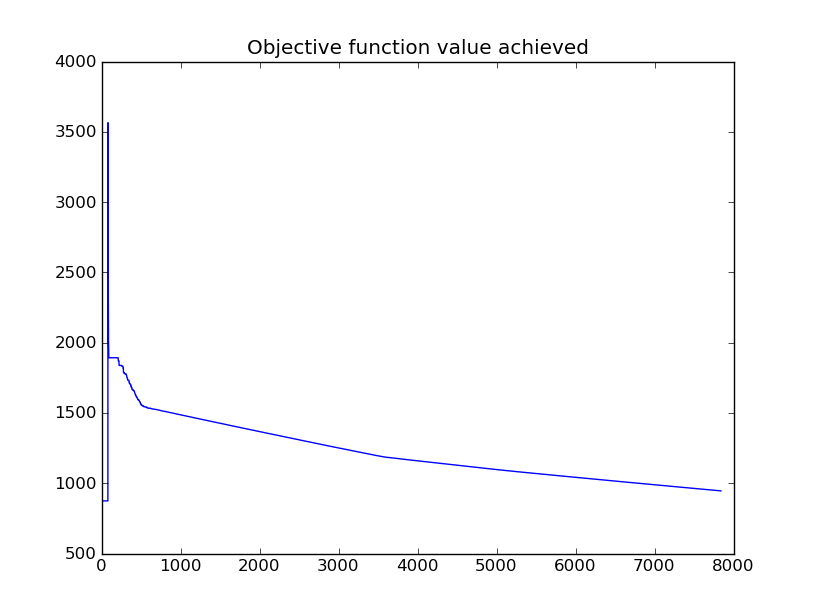
I modified the Nelder Mead algorithm I wrote for Class 10 to allow for bounds on the design variables. Design variables are the ones that the algorithm modifies as it seeks a minimum of the objective function. Two vectors, of upper bounds and lower bounds, are specified. Any time the algorithm generates a new point for the simplex, it checks to see if its values are within these bounds. If not, the bound-violating values are replaced with the value of the bound. Since the problem I am trying to solve is highly spatial, it made intuitive sense to impose some spatial boundaries. The first test was to optimize the very simple two-beam structure. The objective is the internal strain energy of the structure, which is the product of the nodal forces times the nodal displacements. the design variables are the nodal coordinates of the unsupported node and the cross-sectional area and moment of inertia of the elements. Starting from straight configuration, the algorithm moves the central node up as far as it is allowed, and increases the element size to the upper bounds. This is not surprising - the changes in geometry and the increased element stiffnesses both reduce displacement of the node, reducing internal strain energy. The start and end points of the optimization, as well as a time history of the best objective achieved in each simplex, are shown in the figure below.
Relevant Source Code:
SearchAlgorithms.py contains the code for the Nelder Mead algorithm. Note that there are two classes - NelderMeadConstrained and NelderMead. The constrained version includes a penalty formulation for handling constraints, and is not used in this example.
Program_Simple_1.py contains the code that generates the initial structure and sets up the optimization
Notes:
- The geometry variables have a tendency to "stick" to the boundary once they hit it.
- Scaling of the variables was performed. The element sizing values and the geometry values can differ by up to two orders of magnitude. The simplex (and of the upper and lower bounds) is scaled so that all values are of the same order of magnitude. When the calls to the objective function are made, the variables in the simplex are scaled back up to their real values before being passed to the Structure object
4. Displacement-Constrained Minimization of a Simple Structure
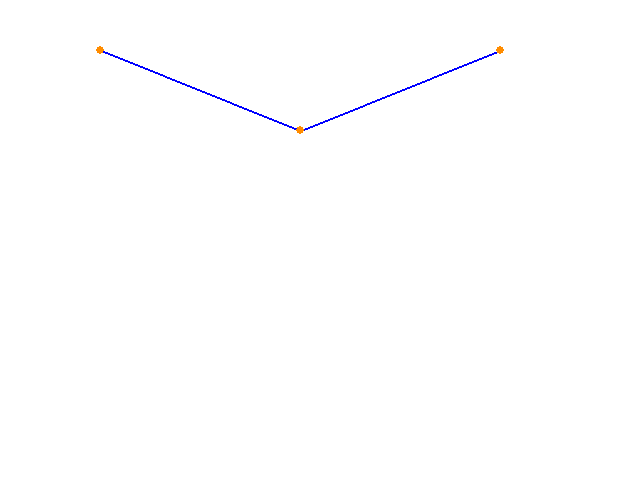
Next, I formulate a different objective function to be minimized - the volume of the frame. As before, the optimization algorithm modifies the geometry of the structure and the cross sectional properties of the structural elements. Using the unconstrained algorithm as before produces results that are, predictably, not very useful. Considering that volume is the product of area and length, the algorithm moves the geometry so that the three nodes are collinear, minimizing the sum of lengths, and reduces the cross sectional area until it hits the imposed lower bound. This is what we would expect a minimizing algorithm to do, but it results in a structure that exhibits enormous displacements. This motivates the inclusion of a set of constraints on the displacements of the nodes. After a search through the literature on applying Nelder Mead to structural optimization problems I elected to use a penalty method with an adaptive penalty term, following the work of Luersen et al. Each time a constraint is violated, its penalty term is increased. Appendix B of the linked paper explains why this works. I do not implement the probabilistic restart part of their work.
Applying this version of the optimization algorithm to the simple structure shows good results. The algorithm broadly minimizes lengths and reduces cross sectional areas, but the displacements of the nodes are not allowed to exceed a prescribed value.
Relevant Source Code:
SearchAlgorithms.py contains the code for the Nelder Mead algorithm. This time, the constrained version, using a penalty method with adaptive linear penalty terms, is used.
Program_Simple_2.py contains the code that generates the initial structure and sets up the optimization. Displacement limits and penalty knobs are set here
Notes:
- It looks like the value of the objective function got worse over time. What is actually happening here is that every time the penalty multipliers increase, the objective function changes. So the apparently worse points later in the series were evaluated against an objective function with higher penalty terms. It would be more useful to look at the time history of the original function (subtracting out the penalty terms)
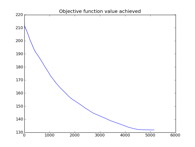
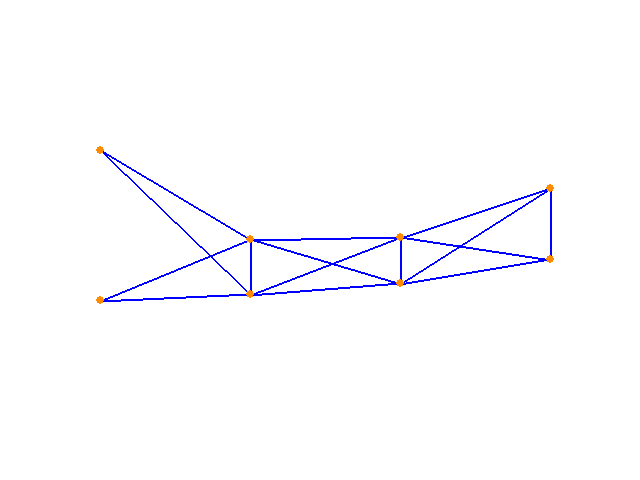
5. Optimization of a more complex structure
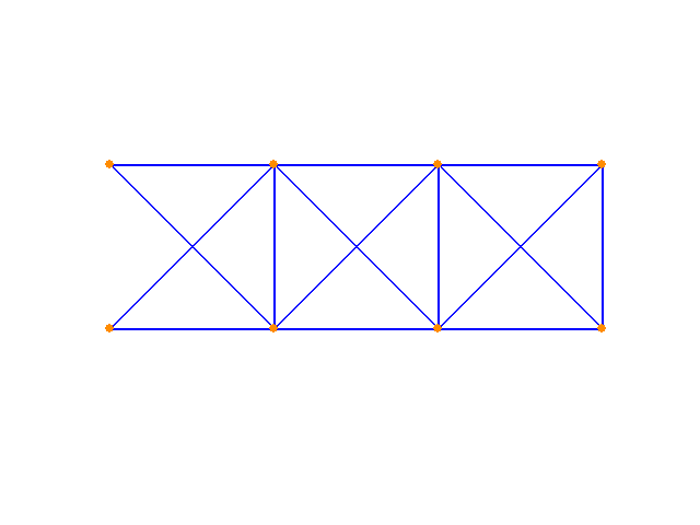
Having established that the method is working for the simple structure, the next challenge is to apply it to a more complex assemblies. The following images show the optimization of strain energy. Only the y-coordinates of the nodal geometry (and not the element properties) are allowed to vary.
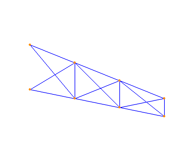
Now, the member properties are allowed to vary along with the geometry y-coordinates. Again, the algorithm seeks the solution that minimizes strain energy. A range of starting points end in the same solution, shown below:
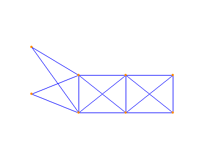
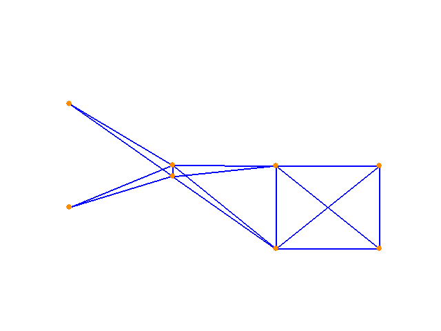
And finally, applying the constrained version of the algorithm to the same structure in pursuit of the minimum volume structure (with a displacement limit imposed):

Relevant Source Code:
Program_Complex_1.py contains the code that generates the initial structure and sets up and runs the energy optimization.
Program_Complex_2.py does the same thing for the volume minimization.
Notes:
- Optimization gets pretty slow for this structure, taking on the order of a minute to complete
- It's important to remember that the cross sectional area and the moment of inertia for each element are also decided by the algorithm, although the visualizations above do not show i. The problem size is considerably larger than one might assume from merely looking at the images.
6. Making Use of Gradients
Everything so far has implicitly assumed that the structural model is a black box, and that I do not know anything about the structural equations I'm solving. This, of course, is not the case. The FEM analysis I implemented is the solution to a set of equations. I can write these equations down and differentiate them to find the gradient of the objective function with respect to the design variables. This will allow me to use a gradient-based search method which should exhibit better performance than Nelder Mead. Note that the analysis requires the inversion of the stiffness matrix of the structure. A naive first approach would be to attempt to find the derivative of the inverse of this matrix, an extremely tedious task which would be impractical to easily implement for more than a single example of a structure. A more nuanced approach is given in Fox's Optimization Methods for Engineering Design (Fox, 1971). This formulation is discussed here.
7. Some additional comments
Part of the challenge I set myself in doing this project was to gain familiarity with object-oriented programming in Python. Everything I have done here is in a class, and I have tried to use everything I already know about OOP to make well-organized, reusable code. Python is pretty different to C# or Java in this regard, but some of the differences offer great flexibility and let me do things that would be more complicated in Java. I found the ability to attach methods to objects at runtime quite useful, although a little messy. I used this to define a method that updated the structure based on a change in design variables. It is much more natural to change this in the code that runs the optimization, rather than modifying the structure class every time I want to change the design variables. There are plenty more examples of this kind of thing. On the whole, I'm glad to see that Python is a viable way to write object-oriented code, brining with it all the additional benefits of writing in Python such as quick development time and wide availability of libraries and bindings
© Rory Clune 2011