
The inverted-pendulum system is a classic example of an unstable mechanical system. It has been tackled using many different approaches. In this project my aim is to simulate an inverted pendulum using Javascript and design a state space controller to balance the pendulum. I also plan to investiaget merits of a data-driven approach over a classical control system, based on metrics of development time and robustness.
Classical control involves creating at model of a system (typically called the 'plant') and combining this with a control system. For example, a propellor mounted on a shaft that can rotate around a central point, a simple model might contain a relationship between the current supplied to the motor and the resulting angle of the shaft. To create a more accurate model of the system, features such as the motor resistance and air resistance must be factored in. This classical approach for designing the controls of a system is sufficient for a large number of applications however there are clear limitations in gaining a truely accurate model. Alternative data driven approaches are being used to design controllers for systems such as the inverted pendulum without providing any model of the system.
To begin with I modifed the Runge-Kutta method that we worked on earlier in the semester to simulate an inverted pendulum given a sinusoidal, horizontal disturbance. To do so the equations of motion are required. These can be developed using the Lagrangian method, where T is the kinetic energy and U is the potential energy:
$${L = T - U}$$ $${T = \frac{1}{2} m_1 v_1^2 + \frac{1}{2} m_2 v_2^2}$$ $${U = -m_1 g l cos(\theta)}$$ $${v_1^2 = \dot{x}^2}$$ $${v_2^2 = \dot{x}^2 - 2lcos{\dot{\theta}}\dot{x} + l^2\theta^2}$$ $${L = \frac{1}{2} (m_1+m_2) \dot{x}^2 - ml\dot{x}\dot{\theta}cos{\theta} + \frac{1}{2}ml^2\theta^2 - mgsin(\theta)}$$The Lagrangian equations applied to this system are:
$${\frac{d}{dt} (\frac{\partial L}{\partial\dot{x}}) - \frac{\partial L}{\partial x} = F}$$ $${\frac{d}{dt} (\frac{\partial L}{\partial\dot{\theta}}) - \frac{\partial L}{\partial \theta} = 0}$$If you do the derivatives and plug everything in then you get the following equation of motion:
$${m \ddot{x} cos(\theta) + ml\ddot{\theta} = mgsin(\theta)}$$Solve using a 4th order Runge-Kutta:
$${y_1 = \theta~~\ddot{y_1} = \dot{\theta}}$$ $${y_2 = \dot{\theta}~~\dot{y_2} = \ddot{\theta}}$$Substituting into the governing equation
$${m \ddot{x} cos(\theta) + m l \dot{y_2} = mgsin(\theta)}$$Rearranging, we have expressions for the derivatives of ${\theta}$ and ${\dot\theta}$ which are used in the Runge-Kutta update:
$${\dot{y_1} = \dot\theta = y_2}$$ $${\dot{y_2} = \ddot\theta = {gsin(\theta) - \ddot{x}cos(\theta) \over l}}$$Having got the simulation up and running, I added the sliders below to explore help explore the resonant frequency of the system.
Amplitude
3.10Omega
0.26Damping
0.01In the plot above, position = dark purple, velocity=pink and acceleration = light blue. The plot was created using a Smoothie chart.
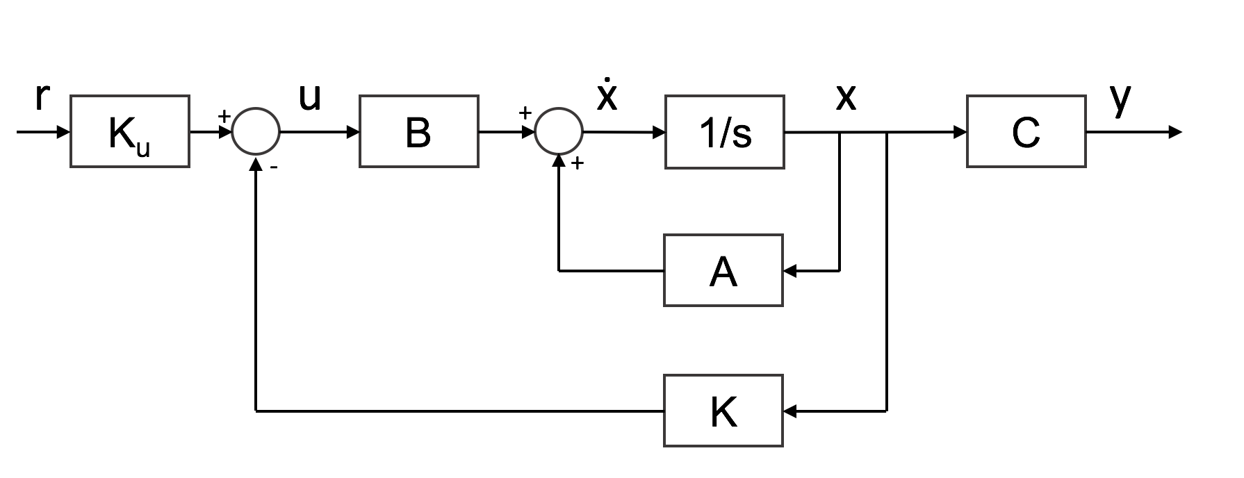
In order to design a control system for the system, it's necessary to add in equations that describe the impact of the dynamics of the base on the pendulum. I followed some notes provided by the University of Michigan and Matlab to develop a Matlab script to describe a closed loop system. The states (X) that are included in this control system are described below.
$$X = \begin{bmatrix}x \\ \dot{x} \\ \theta \\ \dot{\theta} \end{bmatrix}$$ $$p = I(M+m)+Mml^2$$ $$A = \begin{bmatrix}0 & 1 & 0 & 0 \\0 & \frac{-b(I+ml^2)}{p} & \frac{-b(g m^2 l^2)}{p} & 0 \\0 & 0 & 0 & 1 \\0 & \frac{mlb}{p} & \frac{mgl(M+m)}{p} & 0\end{bmatrix}$$ $$B = \begin{bmatrix}0 \\ \frac{I+ml^2}{p} \\0 \\ \frac{ml}{p} \end{bmatrix}$$ $$C = \begin{bmatrix}1 & 0 & 0 & 0 \\ 0 & 0 & 1 & 0\end{bmatrix}$$ $$D = \begin{bmatrix}1 \\ 0 \end{bmatrix}$$These matrices are combined to form a differential equation for the system.
$$\dot{X} = AX + BU$$ $$Y = CX + DU$$Where K is a matrix of the gains which are calculated using LQR
$$K = \begin{bmatrix}K_x & K_\dot{x}& K_\theta& K_\dot{\theta} \end{bmatrix}$$U is the input to the system. This setup has one input, the position of the base, therefore U is a scalar value which is calculated using the following equation.
$$U = K_u R - KX$$ $$\begin{bmatrix}u \end{bmatrix} = \begin{bmatrix}Ku_1 & Ku_2 \end{bmatrix} \begin{bmatrix}x_{desired}\\\theta_{desired} \end{bmatrix} + \begin{bmatrix}K_x & K_\dot{x} & K_\theta & K_\dot{\theta}\\ \end{bmatrix} \begin{bmatrix}x\\ \dot{x} \\ \theta \\ \dot{\theta} \end{bmatrix}$$Lastly, R is in the desired state of the system. In the case of this system, the main goal is to keep the pendulum vertical where ${\theta = 0}$ however, in addition to satisfying this condition, it's necessary to place a constraint on the range of motion of the base. Therefore there are two inputs to the system. In a real system there would also be constraints on the velocity of the base, given limits of the motor driving it.
$$R = \begin{bmatrix}0.2 \\ 0 \end{bmatrix}$$In the Javscript simulation, I'm running a discrete time system, therefore, in Matlab, I first discretized the model and then used Linear Quadratic Regulation (LQR) through the Matlab function dlqr() to determine state-feedback control gains. LQR calculates the optimal gain matrix K such that the state-feedback law ${u[n] = -Kx[n]}$ minimises the following quadratic cost function. As mentioned in an earlier part of the project, it's at this point that a search method could be used to determine the Q and R values to minimise the cost function. For now, I have been adjusting the Q and R values based on plots of the impulse and step responses generated in Matlab, like the ones shown below.

It took my a while to get my head around the update loop within the Javscript animate function. Most of the issues were to do with understanding the what dimensions the matrices presented above should have. In future, I'll be sure to be very clear on which variables are inputs and outputs and generate the matrices accordingly. For the main animation loop in Javascript I've ended up doing the following:

Gain for base position
-5.41Gain for base velocity
-8.88Gain for angle of pendulum
76.6Gain for anglular velocity of pendulum
13.01
The next step that I'm interested in is how little you can know about the dynamics of the system when designing a controller. To do this I will try and use Nelder-Mead to search for a function of the input to the system based on previous information about the angle of the pendulum and the movement of the base. To mimic the current controller, the function for the input would need some way to describe position, velocity and acceleration terms for the angle and base position. $$x[n] = a~\theta[n-1] + b~\theta[n-2] + c~\theta[n-3] + d~x[n-1] + e~x[n-2]$$
I need a cost function to evaluate for each set of coefficients. One idea that Sam helped me come up with is a summation of $\theta^2$ and $\dot{\theta}^2$ for n steps of time dt, from p starting positions within the range of d degrees either side of $\theta = 0$. The range D degrees will be kept small to ensure that the function for x[n] will be mapping approximately linear dynamics. I am using the following parameters to get everything running:
$$Starting~positions = p = 10$$ $$Number~of~time~steps = n = 100$$ $$Time~step = dt = 0.01$$ $$Limit~on~range~of~motion = \pm10^{\circ}$$
The cost function is calculated as follows. This is the function evaluated by Nelder Mead.
$$Cost = \sum_{S=1}^{s} \sum_{N=1}^{n}(\theta^2 + \dot{\theta}^2)$$The results below are kind of exciting. They initial set of plots show what happens to the pendulum from 10 different starting points with no form of control, they correctly fall to one side. The set of plots below that show that Nelder-Mead has successfully come up with coefficients to control the pendulum when released from the starting location.
These two plots show the system with an intial set of coefficients [c,-c,c,-c,c] where $c=1.0e^{-3}$. You can see that the angle of the pendulum diverges.

After running Nelder-Mead I got coefficients of [-864.59503912, 271.18955559, 624.50156982, -259.92153225, 299.97512632] which result in stabilization of the pendulum angle for the 25 time steps of 0.01 seconds in an operation range of 10 degrees either side of the vertical.

This code + plots show converance on a solution when searching for a function with 5 coefficients
Now that this is up and running it becomes very easy to add in additional terms to introduce more historical information into the anstatt. I the next examples I have started to explore the types of results that Nelder-Mead produces for a larger amount of time steps and a wider range of motion.Here I added an extra term for the position history, extended the time steps that cost function runs for and widened the angle around which the starting points begin from.
In this next example I increase the number of time steps that the cost function runs to 100. After this length of time, most of the test cases have fallen below the horizontal, therefore I added in an if statement to the cost function to set the velocities of the these cases to zero after this occurs. Again Nelder-Mead seems to produce some interesting results shown in the plots below. The first plot uses an initial guess for the cofficients of [c,c,c,c,c,c] where $c=1.0e^{-3}$.

After running Nelder-Mead I got coefficients of [-210.57633622, 212.45435534, -30.5532717, -270.49688425, 58.00383923, 218.23968636].

In this project I modelled an inverted pendulum and designed and implemented a state space controller. In moving forwards with the simulation I would aim to make it more realistic by adding in constraints on the velocity of the base to mimic limitations of the motor.
Upon completing the state space controller I then investigated searching for a controller with limited knowledge of the dynamics of the system. This method seems to be quite successful at producing a controller for the region immediately around the pendulum's vertical position. Next steps for this would be to implement the controller function with the Nelder-Mead coefficients to see how well it works and subsequently run this technique on a real system. Furthermore, this method would need to be reimplemented in different regions of the pendulum's rotation due to the fact that the equations of motion vary. In it's full implementation on a real system, this method may therefore produce several controller functions for different regions of the pendulum's operation, with each one coming into play depending on the pendulum's angle.
This project has been very challenging, I'm very glad to have had the opportunity practice designing and implementing a state space controller, furthermore, it's be great to combine this with a simulation of the pendulum and it was really cool to see how capable Nelder-Mead is at search for a controller.
Thanks to Neil for making this class exist. Thanks to Sam for asking so many questions about Python and instilling rigour in my approach to matricies. Thanks to Will for also answering many questions and thank you to Professor Jacob White and Joe Steinmeyer in the EECS teaching lab for teaching my feedback control and helping my get my state space controller up and running.