Some key concepts
+ The result should not depend on the algorithm parameters (for example, decreasing a step size should give the same answer).
+ Check the algorithm on a problem with a known exact solution to make sure that it agrees.
+ IEEE numbers: A *32-bit single precision* floating-point number has a 24-bit *mantissa* (fractional part), corresponding to about 7 decimal digits, and a *64-bit double precision* number has 53 bits or about 16 digits.
+ If you know your system has some conservation laws then you should choose variables that automatically conserve them. (Otherwise, your conservation laws will be ignored by the solution, or will need to be explicitly enforced.)
PROBLEM 7.1
What is the second-order approximation error of the Heun method, which averages the slope at the beginning and the end of the interval?
\begin{equation} \underbrace{y(x + h)}_{\text{output}} = \underbrace{y(x)}_{\text{input}} + \frac {h}{2} \{ \underbrace{f(x,y(x))}_{\text{start slope}} + \underbrace{f[x + h, y(x) + hf(x,y(x))]}_{\text{end slope}} \} \end{equation}Taylor expansion of the end slope:
\begin{equation} \begin{aligned} & f[x + h, y(x) + hf(x,y(x))] \\[3pt] = \; & f(x,y(x)) + h \frac{d}{dh} f[x+h, y(x) + hf(x,y(x))]_{h\,=\,0} + \mathcal{O}(h^2) \\[3pt] = \; & f(x,y(x)) + h \left[ \frac{\delta f}{\delta x} + f(x,y(x)) \frac{\delta f}{\delta y} \right] + \mathcal{O}(h^2) \end{aligned} \end{equation}Substituting:
\begin{equation} \begin{aligned} y(x+h) &= y(x) + \frac{h}{2} \left\{ 2f(x,y(x)) + h\left[ \frac{\delta f}{\delta x} + f(x,y(x)) \frac{\delta f}{\delta y}\right] + \mathcal{O}(h^2)\right\} \\[3pt] &= y(x) + hf(x,y(x)) + \frac{h^2}{2}\left[ \frac{\delta f}{\delta x} + f(x,y(x)) \frac{\delta f}{\delta y}\right] + \mathcal{O}(h^3) \end{aligned} \end{equation}
PROBLEM 7.2
For a simple harmonic oscillator $$ y"+y = 0 $$ with initial conditions $$ y(0) = 1, y'(0) = 0$$ find \( y(t) \) from t = 0 to 100π. Use an Euler method and a fixed-step fourth-order Runge–Kutta method. For each method check how the average local error & the error in the final value and slope depend on the step size.
We can re-write the original equation as:
\begin{equation} \begin{aligned} \ddot y(x)+y(x) &= 0 \\ y(x) &= - \ddot y(x) \end{aligned} \end{equation}
We know that
\begin{equation} \begin{aligned} y(x+h) &= y(x) + h f(x, y(x)) \\ y(x+h) &= y(x) + h \dot y(x) \\ \end{aligned} \end{equation} Similarly \begin{equation} \begin{aligned} \ddot y(x+h) &= \dot y(x) + h \ddot y(x) \\ \ddot y(x+h) &= \dot y(x) + h (-y(x)) \end{aligned} \end{equation}
Euler with error:
t_start = 0
t_end = 100 * math.pi
h = 0.0001

def euler(t_start, t_end, h):
    y_prev = 1
    dy_prev = 0

    y = [y_prev]
    error = [0]

    for i in np.arange(t_start, t_end, h):
        y_new = y_prev + h*dy_prev
        dy_new = dy_prev - h*y_prev

        y_prev = y_new
        dy_prev = dy_new
        y.append(y_new)
        error.append(abs(math.cos(i) - y_new))

    return (np.array(y), np.array(error))

t_start = 0
t_end = 100 * math.pi
h1 = 0.0001

(y_vals, euler_error) = euler(t_start, t_end, h1)
print(np.sum(euler_error)/(t_end/h))
print(abs(y_vals[-1] - math.cos(t_end)))

plt.plot(y_vals)
plt.show()

h2 = 0.1

(y_vals, euler_error) = euler(t_start, t_end, h2)
print(np.sum(euler_error)/(t_end/h))
# 0.0050276672954275075 for h = 0.0001
# 5.0276672954275075 for h = 0.1

print(abs(y_vals[-1] - math.cos(t_end)))
# 0.015831982938209643 for h = 0.0001
# 0.015831982938209643 for h = 0.1

plt.plot(y_vals)
plt.show()
With Runge-Kutta:
t_start = 0
t_end = 100 * math.pi
h = 0.1

def runge_kutta(t_start, t_end, h):
    y_prev = 1
    dy_prev = 0

    y = [y_prev]
    error = [0]

    for i in np.arange(t_start, t_end, h):
        # find kn_y and kn_dy
        k1 = (h*dy_prev, - h*y_prev)

        k2 = (h*(dy_prev+k1[1]*0.5), -h*(y_prev + k1[0]*0.5))

        k3 = (h*(dy_prev+k2[1]*0.5), -h*(y_prev + k2[0]*0.5))

        k4 = (h*(dy_prev+k3[1]), -h*(y_prev + k3[0]))

        # increment y and dy
        y_prev = y_prev + k1[0]/6.0 + k2[0]/3.0 + k3[0]/3.0 + k4[0]/6.0
        dy_prev = dy_prev + k1[1]/6.0 + k2[1]/3.0 + k3[1]/3.0 + k4[1]/6.0

        y.append(y_prev)

        error.append(abs(math.cos(i) - y_prev))

    return (np.array(y), np.array(error))

(y_vals, rk_error) = runge_kutta(t_start, t_end, h)
print(np.sum(rk_error)/(t_end/h))
# 0.06355217587022374 for h = 0.1

print(abs(y_vals[-1] - math.cos(t_end)))
# 0.000840724185820596 for h = 0.1

plt.plot(y_vals)
plt.show()
Runge-Kutta
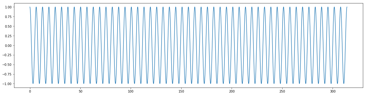
Figure 2
Adaptive Runge-Kutta:
t_start = 0
t_end = 100 * math.pi
h = 0.1

def runge_kutta_step(h, (dy_prev, y_prev)):
    k1 = (h*dy_prev, - h*y_prev)

    k2 = (h*(dy_prev+k1[1]*0.5), -h*(y_prev + k1[0]*0.5))

    k3 = (h*(dy_prev+k2[1]*0.5), -h*(y_prev + k2[0]*0.5))

    k4 = (h*(dy_prev+k3[1]), -h*(y_prev + k3[0]))

    # increment y and dy
    y_prev = y_prev + k1[0]/6.0 + k2[0]/3.0 + k3[0]/3.0 + k4[0]/6.0
    dy_prev = dy_prev + k1[1]/6.0 + k2[1]/3.0 + k3[1]/3.0 + k4[1]/6.0

    return (y_prev, dy_prev)

def runge_kutta_adaptive(t_start, t_end, h):
    y_prev = 1
    dy_prev = 0
    err_thld = 0.01
    step_change_factor = 0.5
    t = 0
    min_step = 0.0001

    y = [y_prev]
    error = [0]

    while t <= t_end:
        # find kn_y and kn_dy
        y_new, dy_new = runge_kutta_step(h, (dy_prev, y_prev))
        y_half, dy_half = runge_kutta_step(h*0.5, runge_kutta_step(h*0.5, (dy_prev, y_prev)))

        if (abs(y_new - y_half) > err_thld) and (h > min_step):
            h *= step_change_factor
        else:
            h *= (2.0 - step_change_factor)

        y_prev = y_new
        dy_prev = dy_new

        #print(abs(y_new - y_half))
        #print(h)
        y.append(y_prev)

        error.append(abs(math.cos(t) - y_prev))

        t += h


    return (np.array(y), np.array(error))

(y_vals, rk_error) = runge_kutta_adaptive(t_start, t_end, h)
print(np.sum(rk_error)/(t_end/h))
print(abs(y_vals[-1] - math.cos(t_end)))

plt.plot(y_vals)
plt.show()