Wireless Power Transfer:
Measurements & Modeling
Summary
Report
1. Introduction
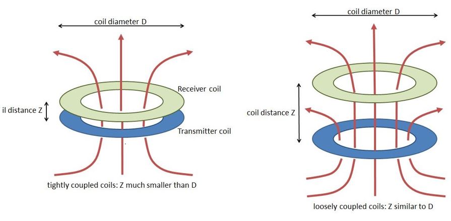
When two inductor coils are placed near each other with their axes aligned, the current applied through coil 1 creates a magnetic field that propagates through coil 2. As a result, a voltage is induced in coil 2 whenever the field strength of coil 1 changes. The voltage induced in coil 2 is similar to the voltage of self-induction, but since it acts upon the external coil 2, it is called mutual induction—the two coils are said to be inductively coupled. The closer the coils are together, the greater the mutual inductance. If the coils are farther apart or are aligned off axis, the mutual inductance is relatively small—the coils are said to be loosely coupled. The ratio of actual mutual inductance to the maximum possible mutual inductance is called the coefficient of coupling, which is usually given as a percentage. The coefficient with air core coils may run as high as 0.6 to 0.7 if one coil is wound over the other, but much less if the two coils are separated. It is possible to achieve near 100 percent coupling only when the coils are wound on a closed magnetic core—a scenario used in transformer design. Mutual inductance also has an undesirable consequence within circuit design, where unwanted induced voltages are injected into circuits by neighboring components or by external magnetic field fluctuations generated by inductive loads or high-current alternating cables. ()
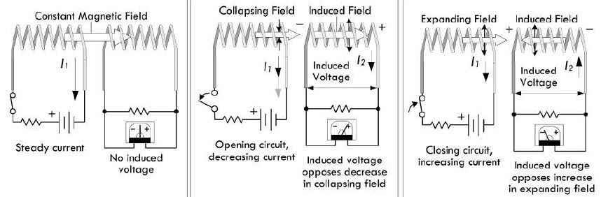
(Source: Monk - Practical Electronics)
As firstly pioneered by Tesla in 1891, wireless power transfer (WPT) has received great interest in the last decade. Wireless power transfer can be either radiative or non-radiative. These two methods are fundamentally based on two different mechanisms: electromagnetic wave and electromagnetic induction. In the radiative case, antennas can emit eletromagnetic power in the form of propagating waves to electric power-consuming devices located at a far distance. For the non-radiative wireless power transfer, it mainly relies on the near-field coupling between two inductive coils, as previously explained. The fast divergence of magnetic field lines restricts pure inductively coupled transfer to operate in such a near range which is generally much shorter than the wavelength of the transmitted power signal. Even so, the inductively coupled transfer has been successfully applied to radio frequency identification (RFID) and wireless charging for some mobile electronic devices nowadays. ( Q. Wu et al. 2015 )
2. Project Goals
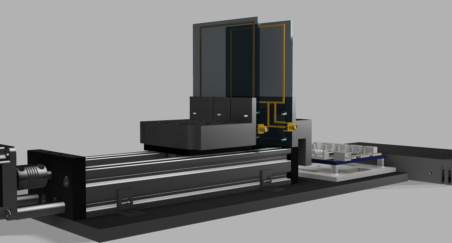
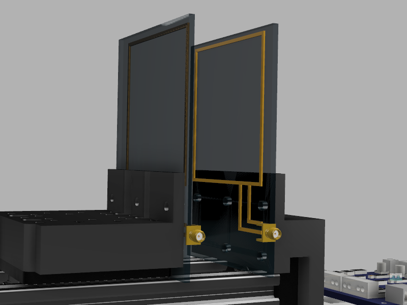
Focusing on the near-field coupling between two inductive coils, the short-term goal of the project is to design
an experimental setup that can recreate this phenomenon using 2 wired coils and measure the transmitted power at different distances using a
Vector Network Analyzer.
In this case, coil 1 creates an alternating magnetic field, then coil 2 receives the corresponding induced electromotive force
by capturing the magnetic field produced from coil 1. According to Faraday’s law of electromagnetic induction, one can easily find
that the induced electromotive force E(t) can be expressed as E (t) = −dϕ/dt = −SμdH/dt, (1) where μ is the effective permeability of
the material contained in coil 2.
Thus, this serves my long term goal of exploring metamaterial architectures such as split-ring resonators
for wireless power transmission. When a time changing magnetic field penetrates through the metallic rings, it induces an EMF by Faraday's Law
electromagnetic induction which in turn produces a rotating current. Because of the current, the ring
its own magnetic field which may enhance or oppose the incident field. Hence there is an inductive
effect associated with the ring.A large number of such split ring resonators are arranged in a periodic array such that EM waves
interact with them as a homogeneous medium. The system has an effective natural frequency which can be tuned
by changing the arrangement of the rings. Thus we can have an effective negative permeability for an adjustable
range of frequencies. Thus, being able to characterize their effective permeability through scattering parameter measurement.
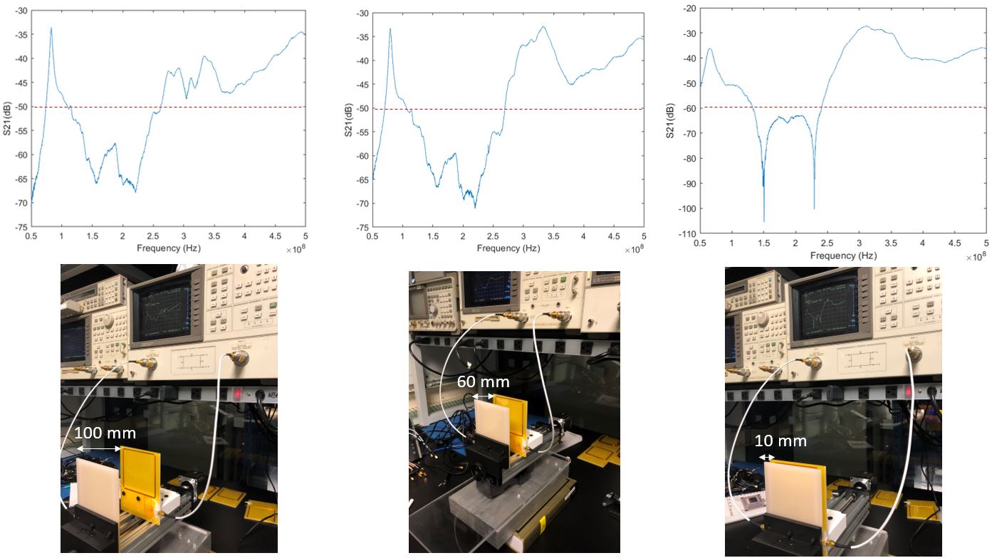
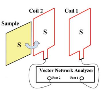
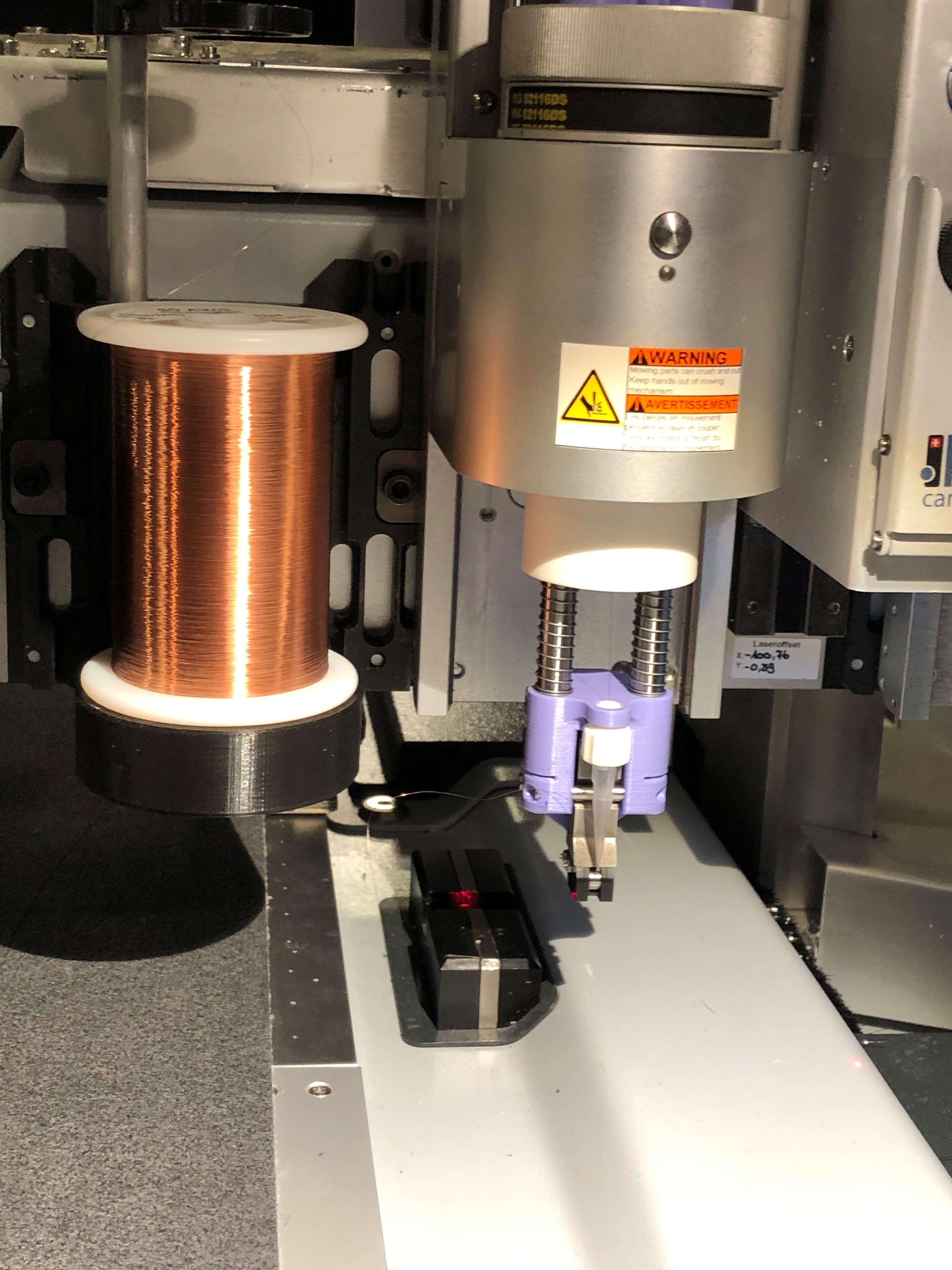
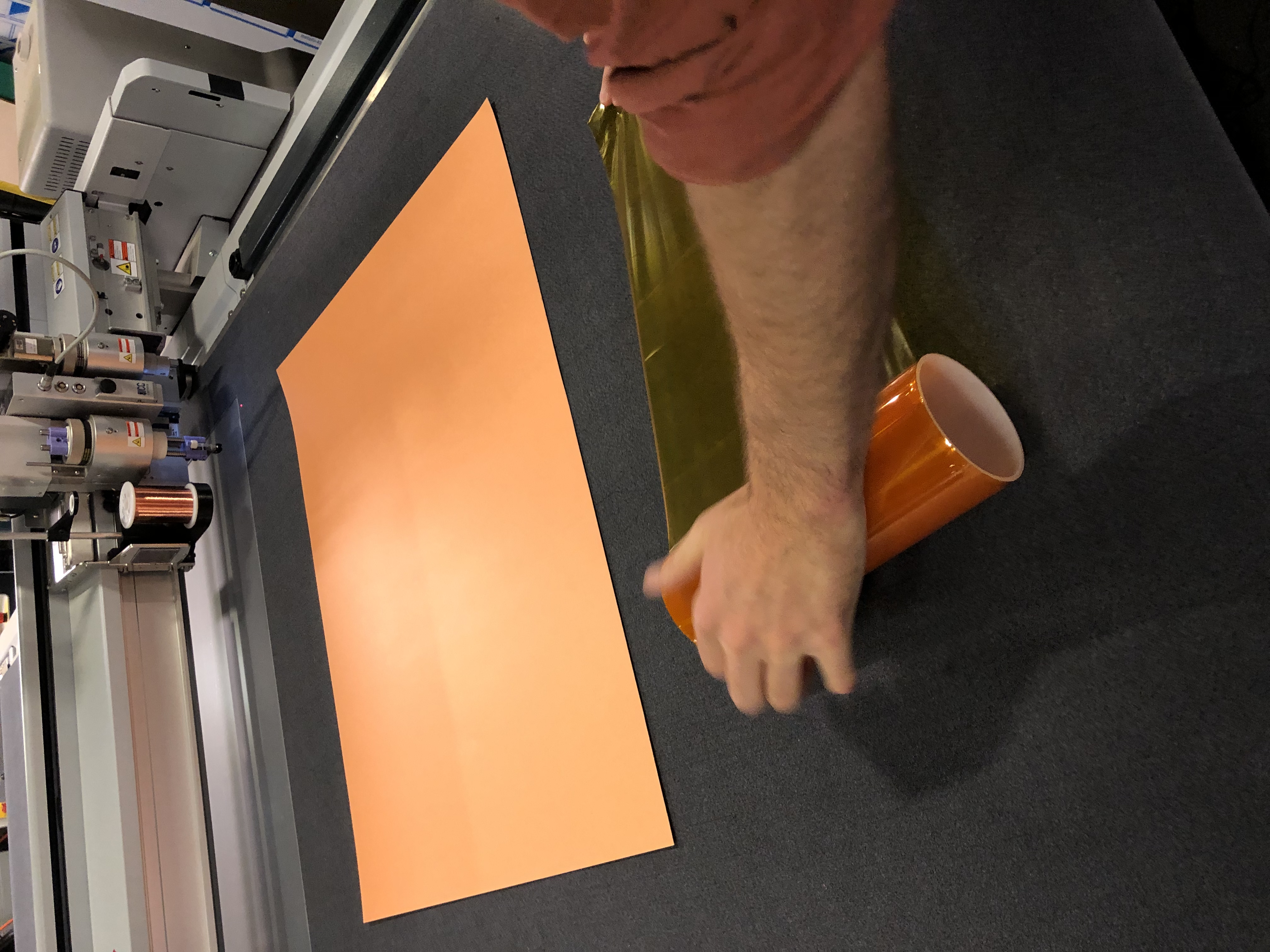
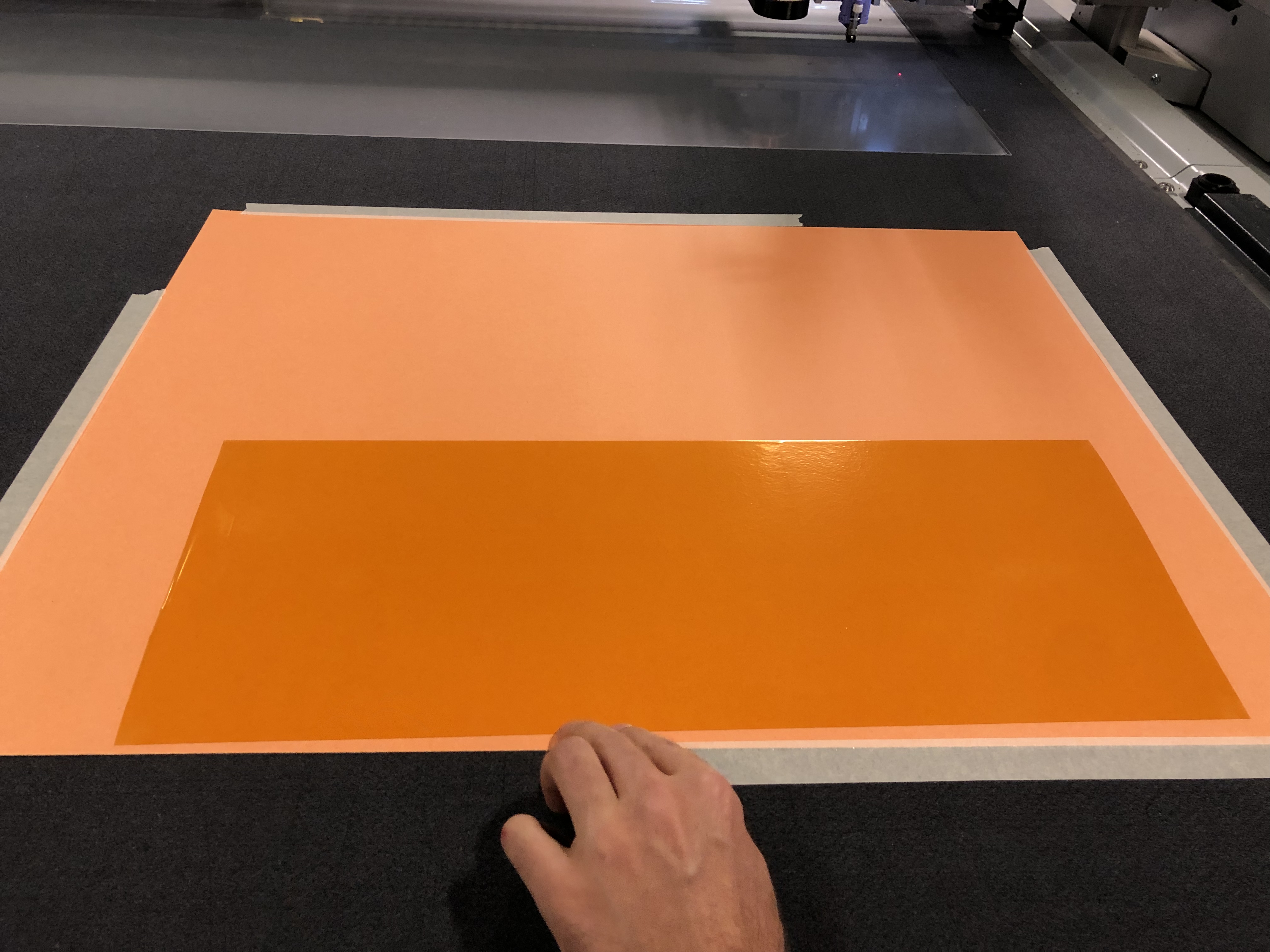
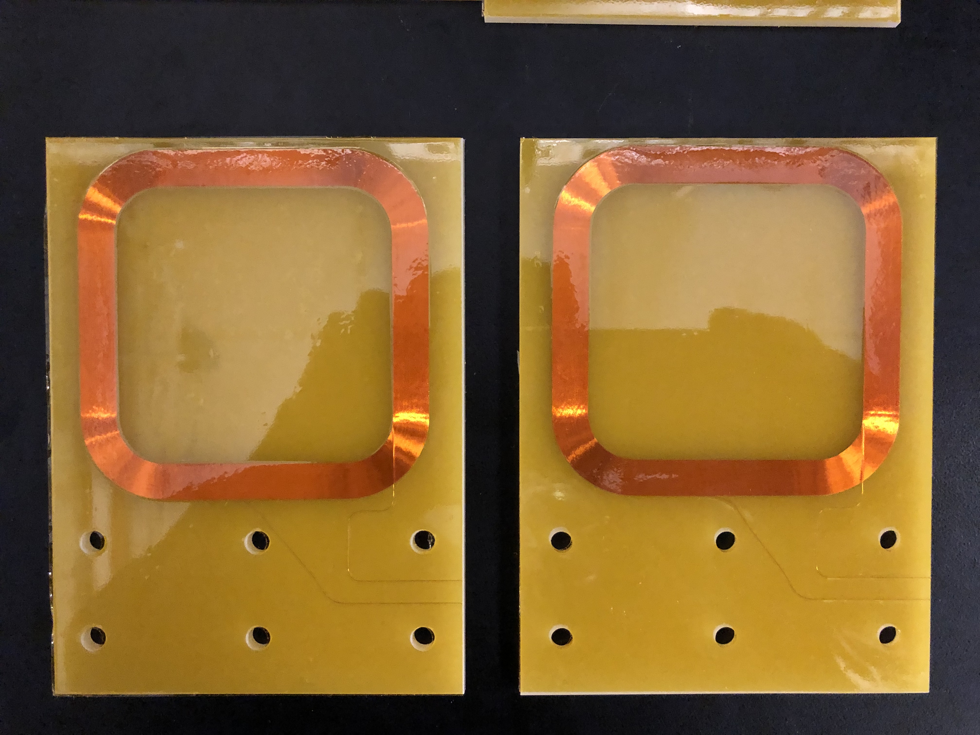
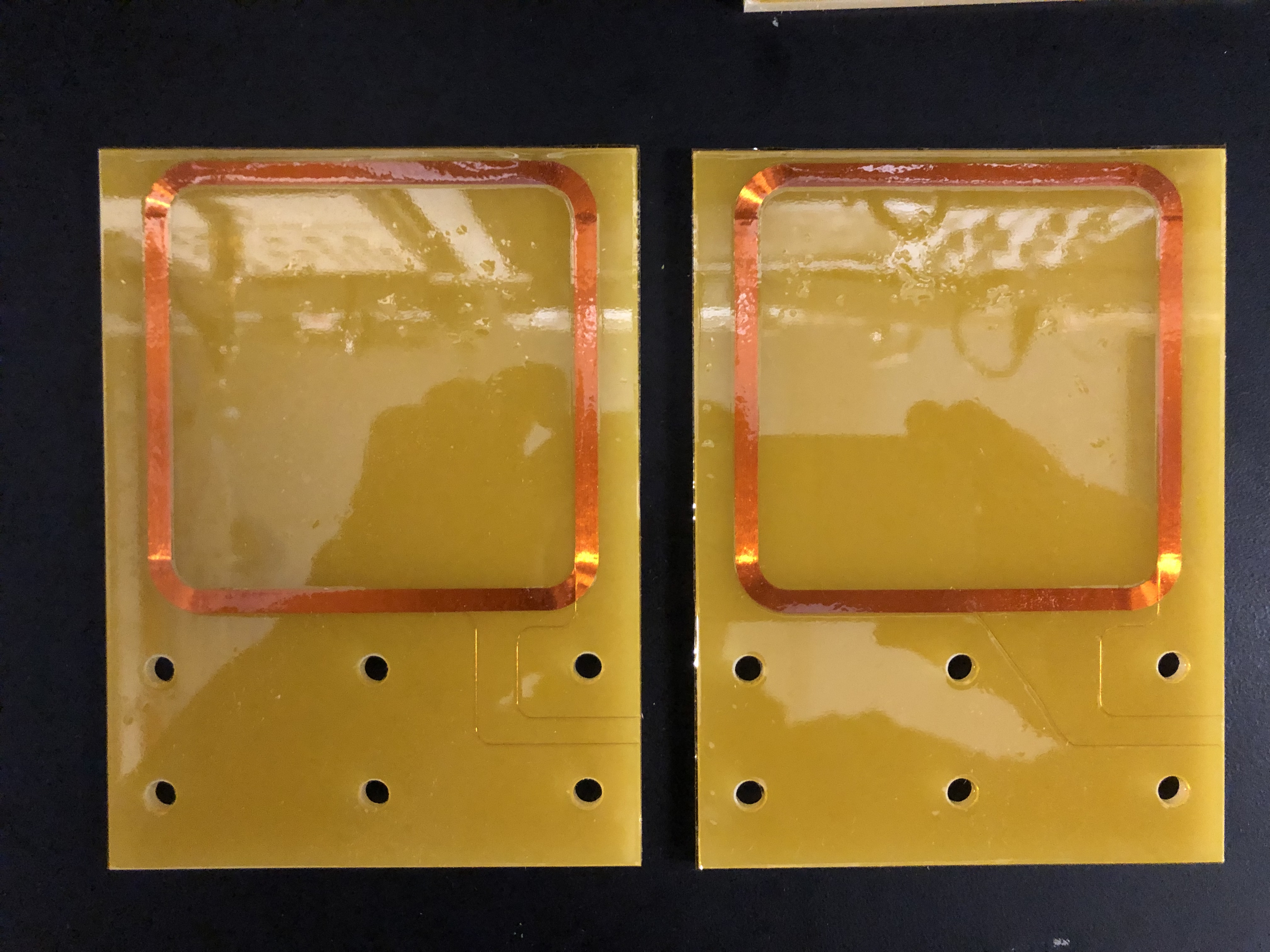
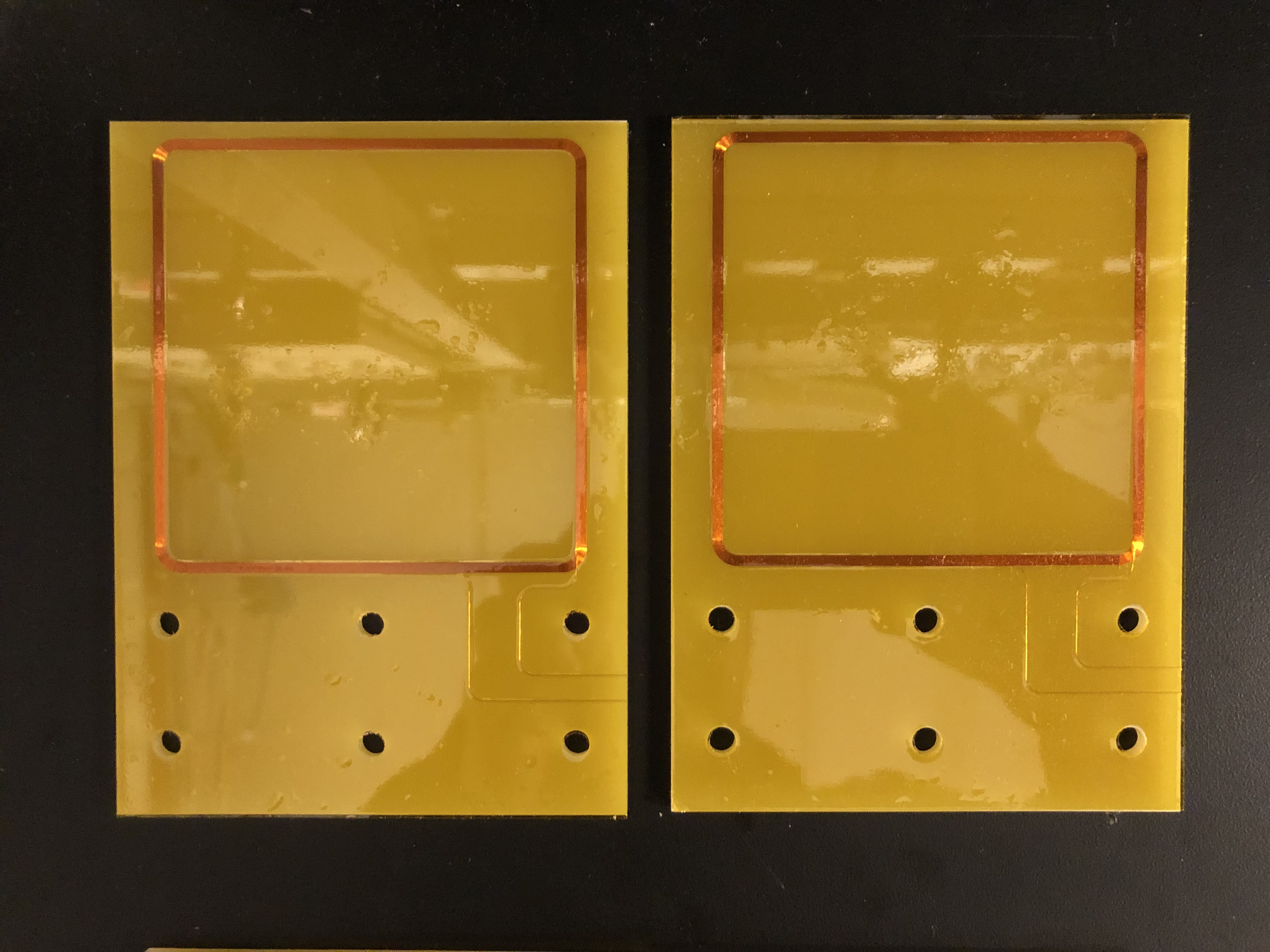
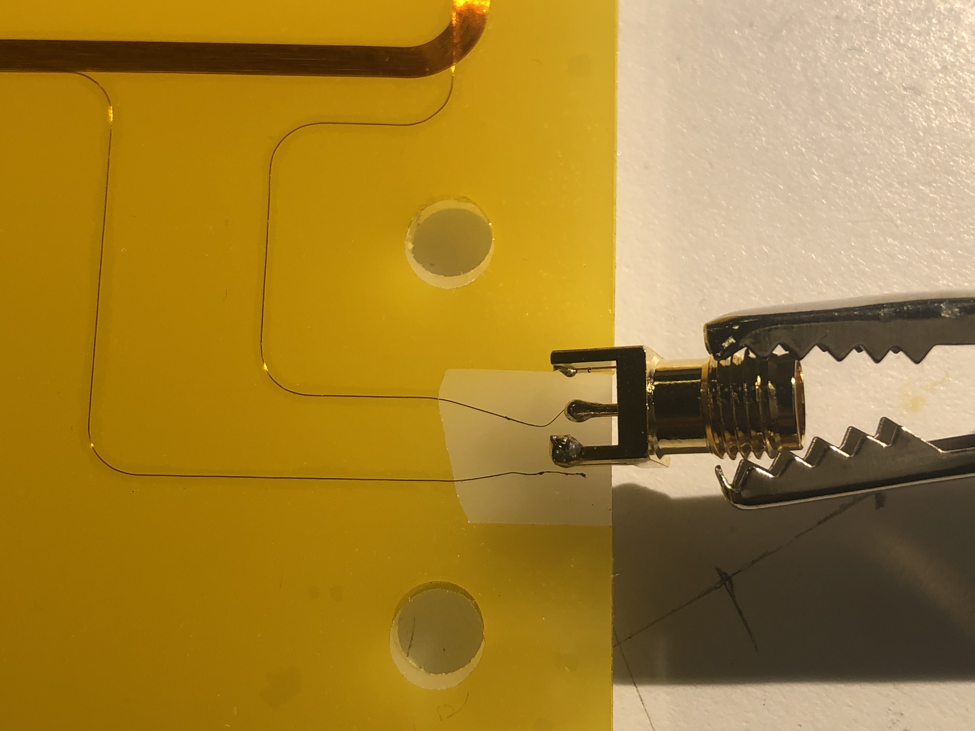
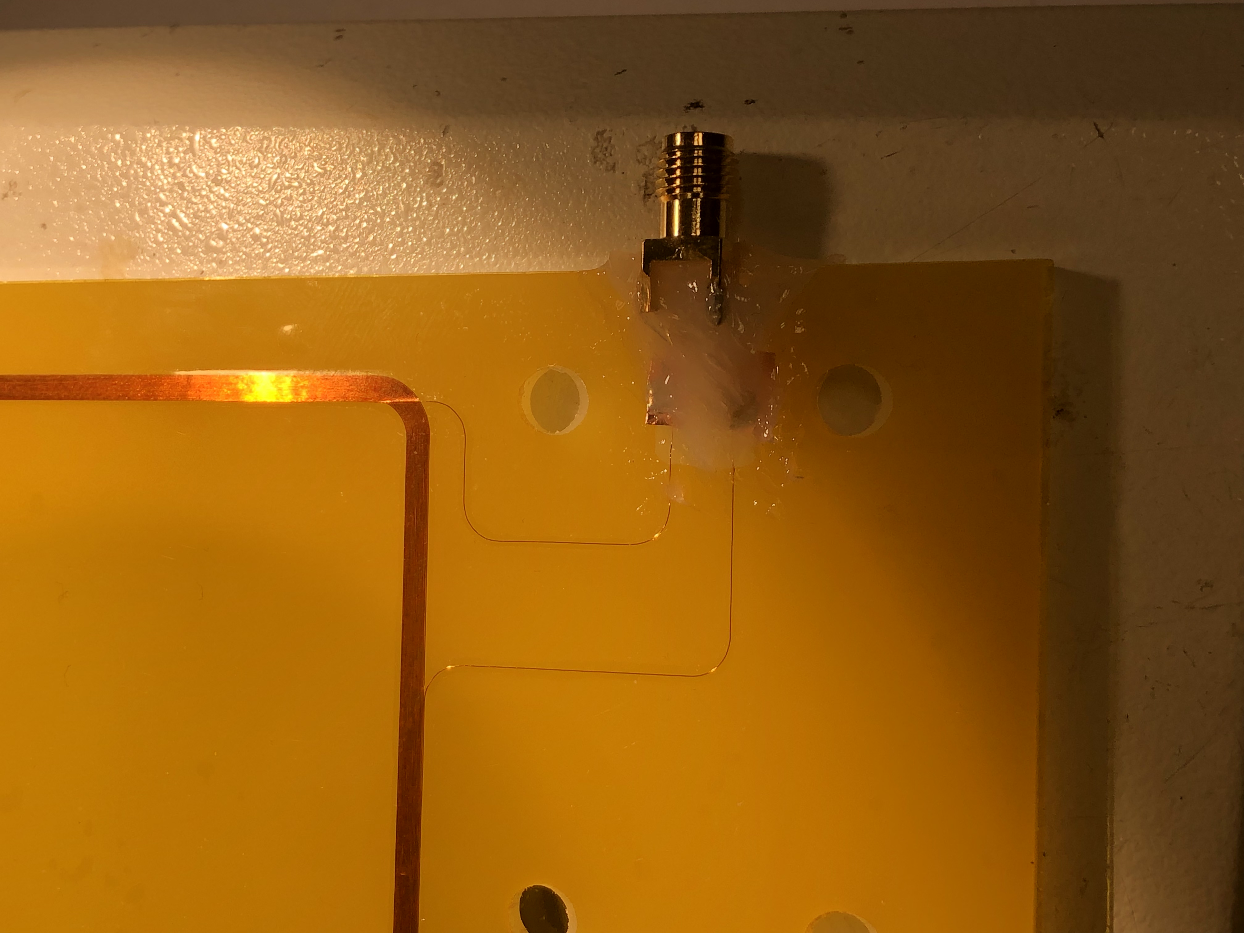
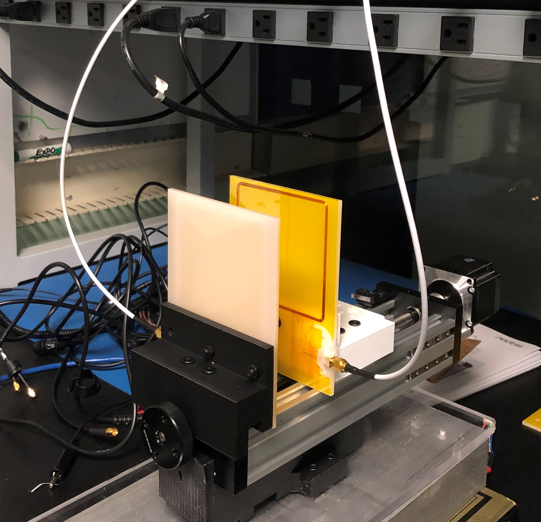
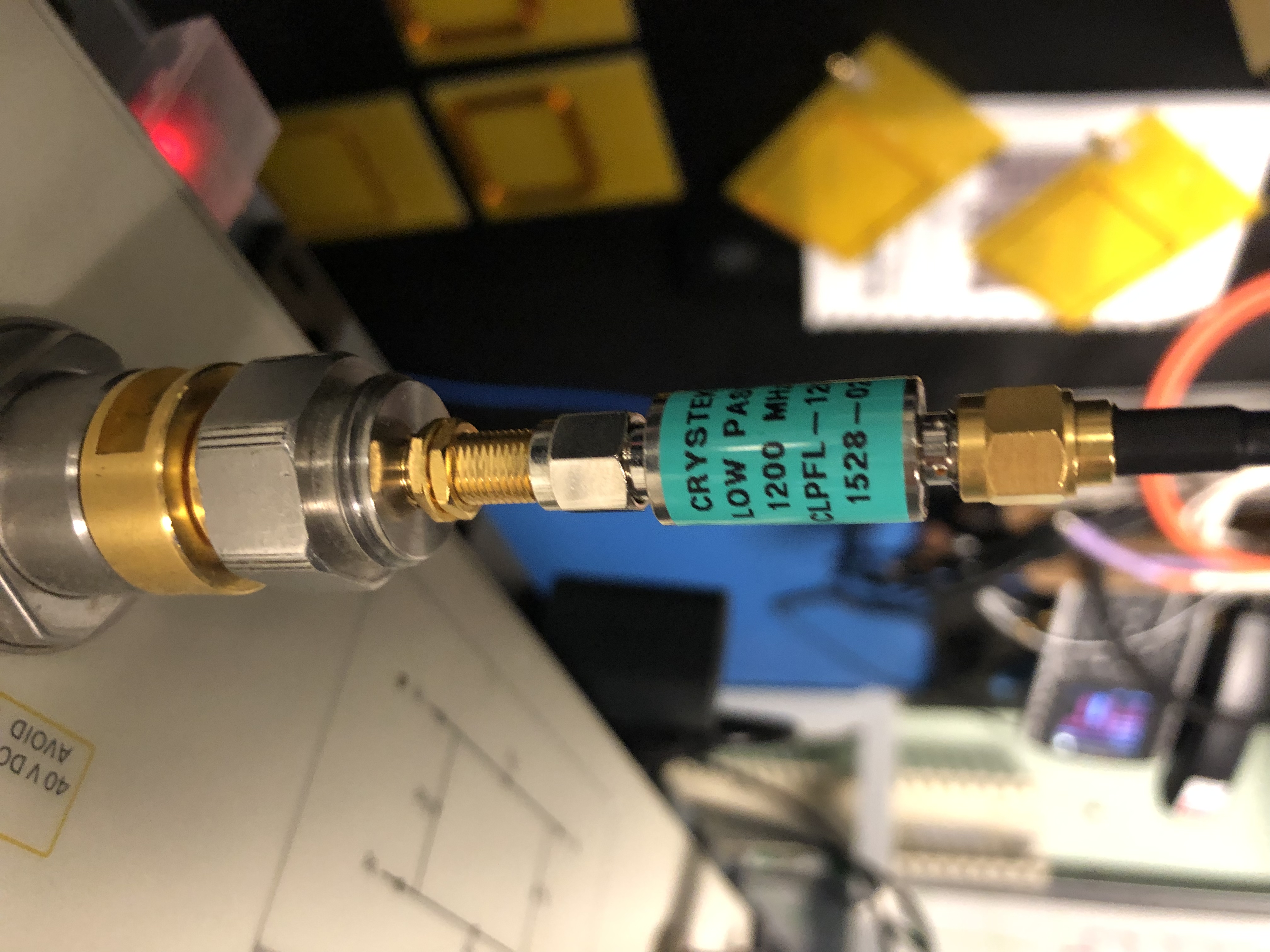
2. Measurements
2-Coil Experimental Setup
....
Coil Plotting (Sam Calisch, CBA)
...
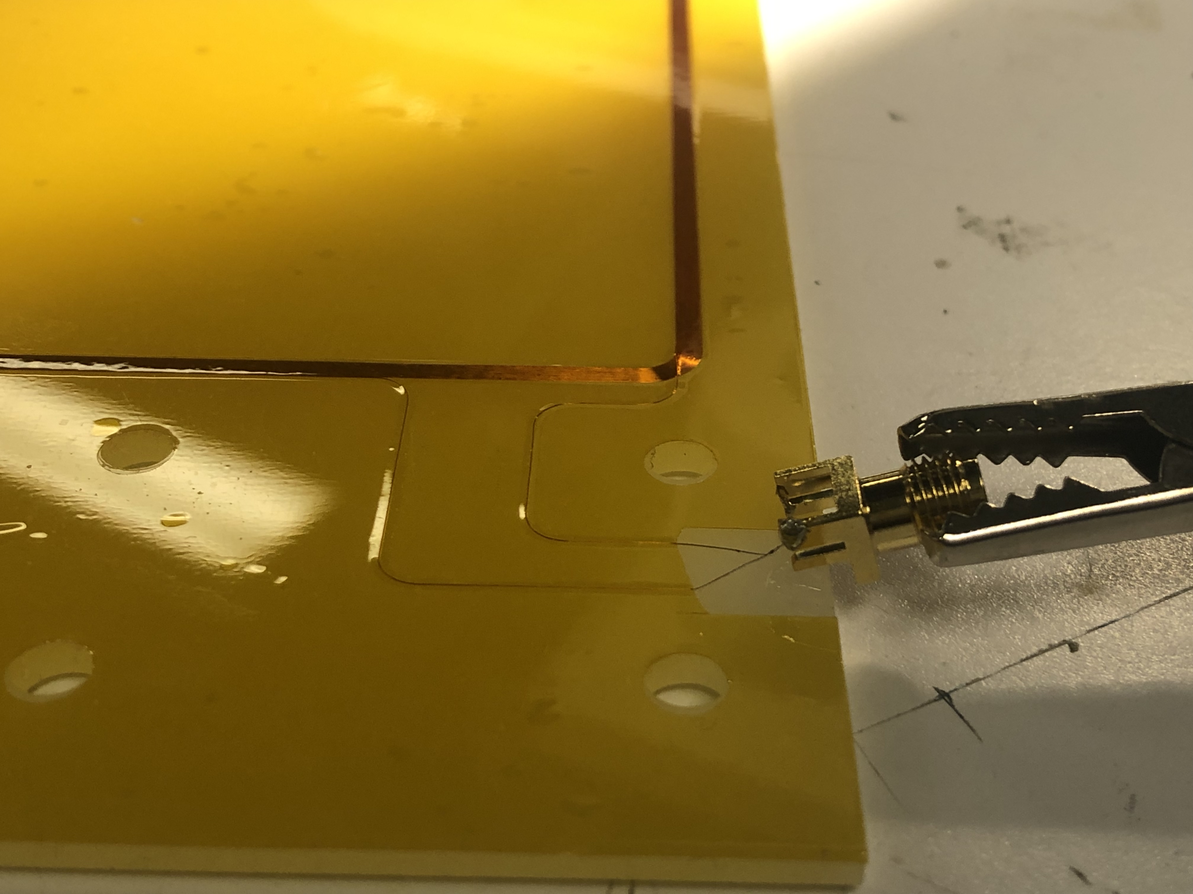

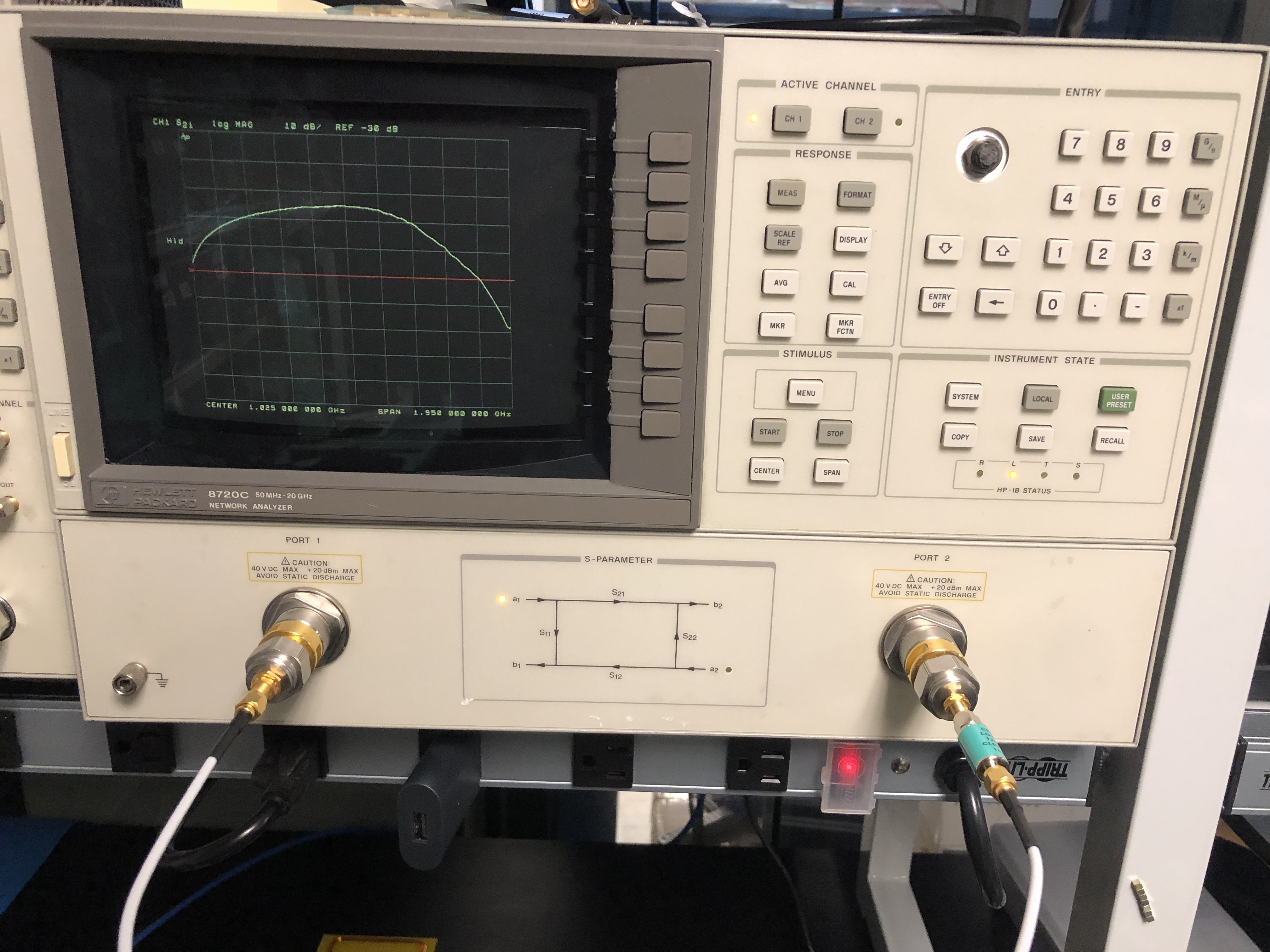
Network Analyzer
S-parameters
Suppose you have an optical lens of some sort onto which you shine a light
with a known photonic output. While most of the incident light passes through the lens, some fraction of
the light is reflected and some is absorbed (the behavior is also dependent on the wavelength of the incident light).
You'd like to characterize that lens: Exactly how much light was reflected? How much passed through? What is it about
the lens that prevented all of the light from passing through?
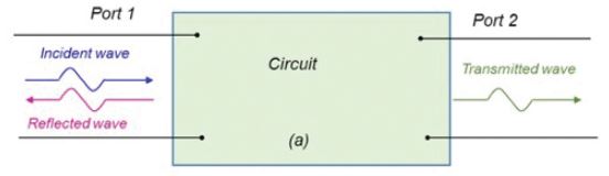
Now, let's apply that same sort of thinking to a two-port network. When we apply a signal to the network's input,
the same thing will happen as it did with the lens: Some fraction of the signal will propagate through the network
but some is reflected, or scattered, back through the port it entered through. Some of the signal will be dissipated
as heat, or even as electromagnetic radiation. As with the lens, we want to know what's happening with our two-port network.
What is causing the scattering of the signal? Bear in mind that the “signal” is an electromagnetic wave propagating through
the medium of the network, just as the light passing through the lens is also an electromagnetic wave.
The answer lies in the application of a mathematical construct called a scattering matrix (or S-matrix), which quantifies
how energy propagates through a multi-port network. The S-matrix is what allows us to accurately describe the properties of
incredibly complicated networks as simple "black boxes". The S-matrix for an N-port network contains N2 coefficients (S-parameters),
each one representing a possible input-output path. By “multi-port network,” we could be referring to, for example, a cable or a
microstrip line. How would that interface affect a 5-Gbps USB 3.0 signal? This is the sort of practical application in which S-parameters shine.
S-parameters are a “frequency-domain” description of the electrical behavior of a network. They are complex numbers, and are
expressed in terms of both magnitude and phase. That's because both the magnitude and phase of the input signal are changed by
the network due to losses, reflections, and propagation time. Quite often we refer to the magnitude only, because how much gain or
loss occurs is typically of the most interest. However, the phase information is extremely important and should not be ignored.
S-parameters are defined for a given set of frequencies and port impedance (typically 50 ohms), and vary as a function of frequency for
any real-world network.
There are also mixed-mode S-parameters. Say you have a differential lane in your circuit and you want to quantify the losses in a differential
signal. S-parameters for the differential lane can be transformed into differential S-parameters, with which you consider differential signal
characteristics alongside of common signal characteristics.
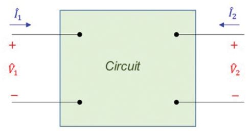
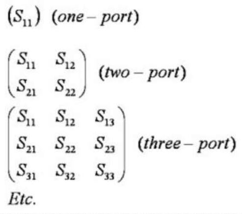
In their most basic sense, S-parameters refer to the ratio of "voltage out versus voltage in." S-parameters come in a matrix, with the number
of rows and columns equal to the number of ports. For the S-parameter subscripts "ij", j is the port that is excited (the input port), and
"i" is the output port. Thus, S11 refers to the ratio of signal that reflects from port one for a signal incident on port one, as a function
of frequency. S-parameters along the diagonal of the S-matrix are referred to as reflection coefficients because they only refer to what happens
at a single port, while off-diagonal S-parameters are referred to as transmission coefficients, because they refer to what happens from one port
to another. Figure 1 shows the S-matrices for one, two, and three-port networks.
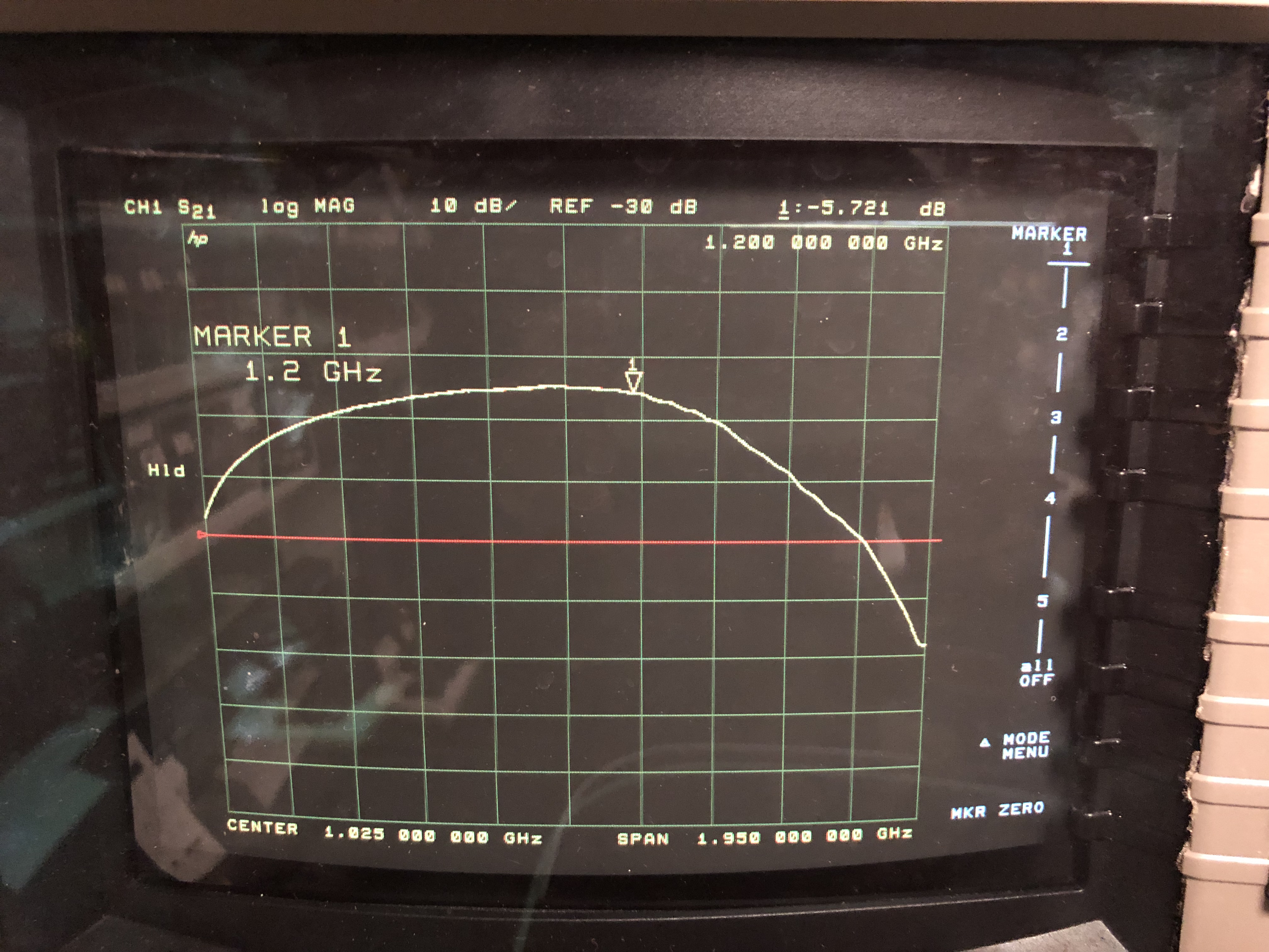
Preliminary Results