NMM: Final Project - Modeling of Discrete Electronics
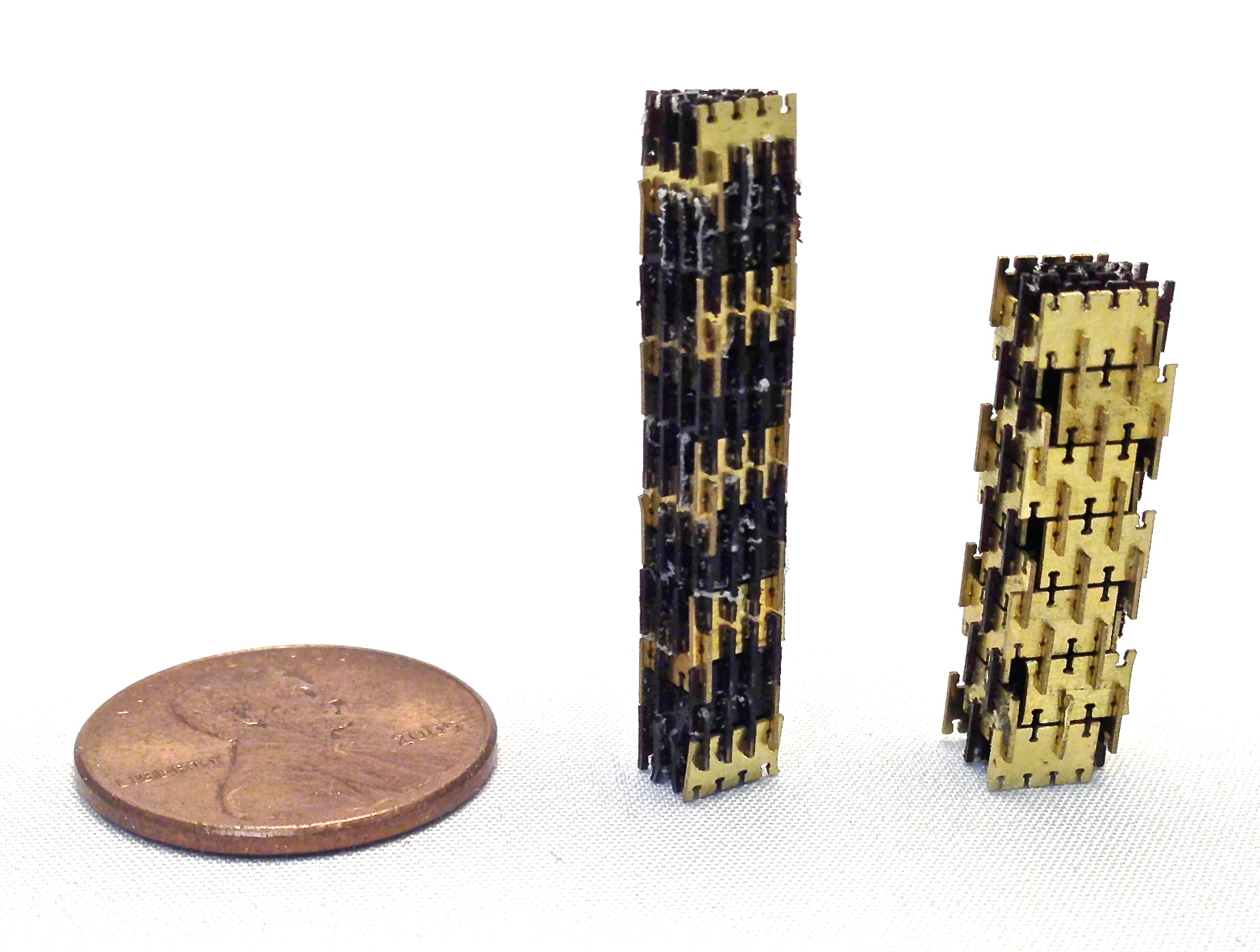
My research involves assembling micro-electronics from pressfit parts. New modeling techniques are required to design and characterize these structures.
My research involves assembling micro-electronics from pressfit parts. Because the structures are inherently three-dimensional, they're not well suited to being designed and modeled in the traditional ways (which, much of the time, assumes relatively planar assemblies. Therefore, new modeling techniques are required to design and characterize these structures. What should these look like?
The Finite Difference Time Domain (FDTD) method for solving elecromagnetic fields is well studied and quite well understood. The most commonly used FDTD algorithm dates back to 1966 when Kane Yee came up with an efficient and more-accurate formulation for Maxwell's equations in a 3D lattice: Yee's Paper (1966). FDTD is now largely used to study and simulate things like sensitive RF circuits, scattering problems, and metamaterials.
There are a number of both commercial and open-source FDTD solvers:
The two references which I found most helpful (and used significantly in this work are):
We'll assume non-magnetic materials ($ \mathbf{H} = (1/\mu_0)\mathbf{B} $) and use this formulation of Maxwell's Equations:
$$ \frac{\partial \mathbf{D}}{\partial t} = \nabla \times \mathbf{H} $$
$$ \mathbf{D} = \epsilon_0 \cdot \epsilon_r \cdot \mathbf{E} $$
$$ \frac{\partial \mathbf{H}}{\partial t} = -\frac{1}{\mu_0}\nabla \times \mathbf{E} $$
But the electric and magnetic constants differ by many orders of magnitude. This could be problematic when we go to implement it on a computer.
$$ \epsilon_0 = 8.85 \times 10^8 \:F/m$$
$$ \mu_0 = 4\pi \times 10^{-7} \:H/m$$
And so we need a change of variables so that E and H on the same order. Let's try changing E to:
$$\tilde{\mathbf{E}} = \sqrt{\frac{\epsilon_0}{\mu_0}} \cdot \mathbf{E}$$
This implies..
$$\tilde{\mathbf{D}} = \sqrt{\frac{1}{\epsilon_0 \cdot \mu_0}} \cdot \mathbf{D}$$
So our update eqations are now:
$$ \frac{\partial \tilde{\mathbf{D}}}{\partial t} = \frac{1}{\sqrt{\epsilon_0 \mu_0}} \nabla \times \mathbf{H} $$
$$ \tilde{\mathbf{D}} = \epsilon_r \cdot \tilde{\mathbf{E}} $$
$$ \frac{\partial \mathbf{H}}{\partial t} = -\frac{1}{\sqrt{\epsilon_0 \mu_0}}\nabla \times \tilde{\mathbf{E}} $$
The Courant condition says we don't want electromagentic waves (which travel at the speed of light, $ c_0 $) to move faster than one unit diagonal per unit time:
$$ \frac{\Delta{t}}{\Delta{x}} = \frac{1}{\sqrt{n} \cdot c_0} $$
For simplicity I use:
$$\frac{\Delta{t}}{\Delta{x}} = \frac{1}{2 \cdot c_0}$$
This makes field updates very simple since $1/ \sqrt{\epsilon_0 \mu_0} = c_0$:
$$\sqrt{\frac{1}{\epsilon_0 \cdot \mu_0}} \frac{\Delta{t}}{\Delta{x}} = c_0 \cdot \frac{1}{2\cdot c_0} = \frac{1}{2}$$
So the simple version of the update equation becomes:
curl_h = (hz[i][j][k] - hz[i][j-1][k] - hy[i][j][k] + hy[i][j][k-1]);
dx[i][j][k] = dx[i][j][k] + 0.5*curl_h;
ex[i][j][k] = gax*dx[i][j][k];
I started by implementing one-dimensional FDTD to get a feel for the structure of the algorithm.
1D FDTD, Gaussian point source, no boundary conditions (left), absorbing boundary (right)

Working my way up, I then implemented the textbook two-dimensional FDTD solver. Here's a plane wave propogating in free space:
For speed I wrote this in C. A python script is passed the name of the C code as an argument and executes bash commands to compile the code, execute it, import the datafile that was generated, and plot or animate it.
Finally, I made a 3D FDTD solver. While the code takes the same form as the two previous implementations, it's significantly more code and uses a pretty good chunk of memory to run. Once I got the bare bones 3D version working I made a number of additions to make the solver practical for EM simulations.
First, I added a Perfectly Matched Layer (PML) absorbing boundary condition. This treats the outermost cells as lossy material that minimizes the reflection of the oncoming wave.

Next, I divided the space into two spaces: the total field and the scattered field. The total/scattered field formulation allows a source generated on one end of the domain to be cancelled out on the other end. This minimizes the load on the PML (to minimize reflections) and allows for simulations of things like scattering parameters from plane wave sources.
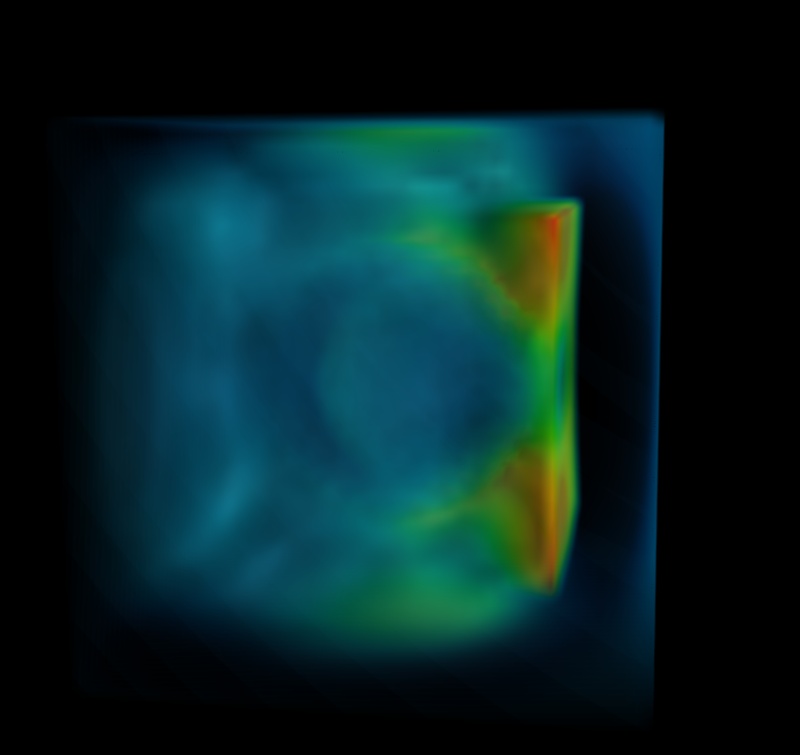
Here I'm showing a plane wave hitting a dipole antenna:
As you can see, I also added the ability to show and animate 3D volumetric data. For this, I'm using Mayavi (and specifically mlab) which can be called straight from the Python wrapper.
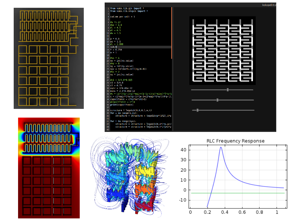
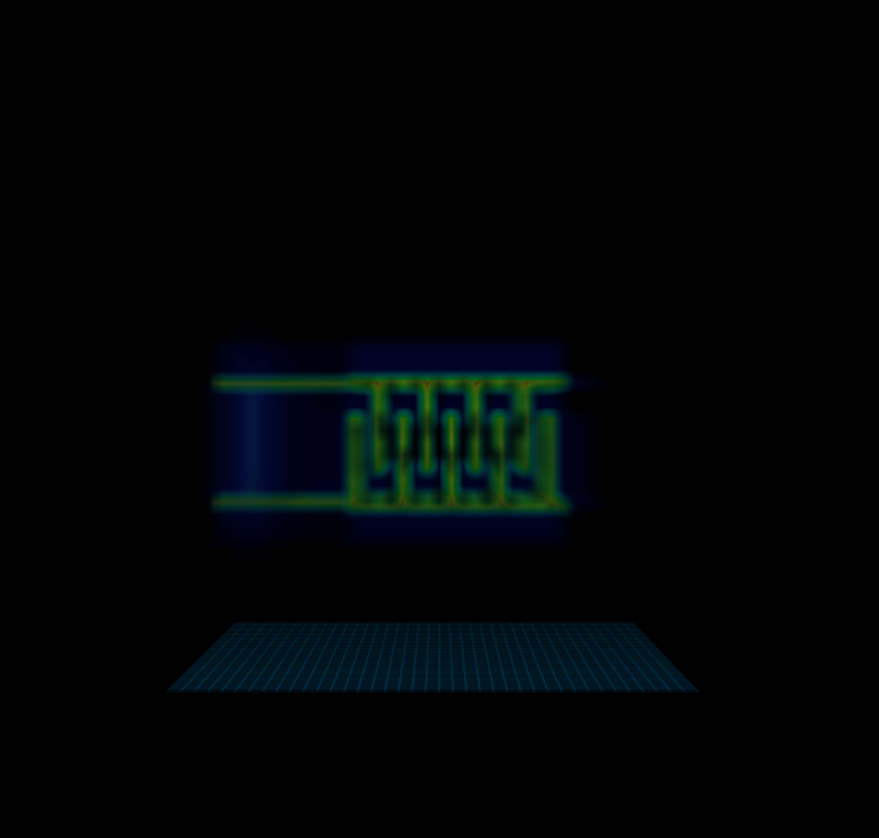
To make it easy to import geometry into the solver, I added the ability to import volumetric data in the form of animated gifs (or stacks of images). So the GIF on the left gets imported and becomes the volumetric data on the right.

Disclaimer: I make no guarantees about the working state of these:
To verify the accuracy of the simulation you can either compare the solution to analytical results or to real measurements.
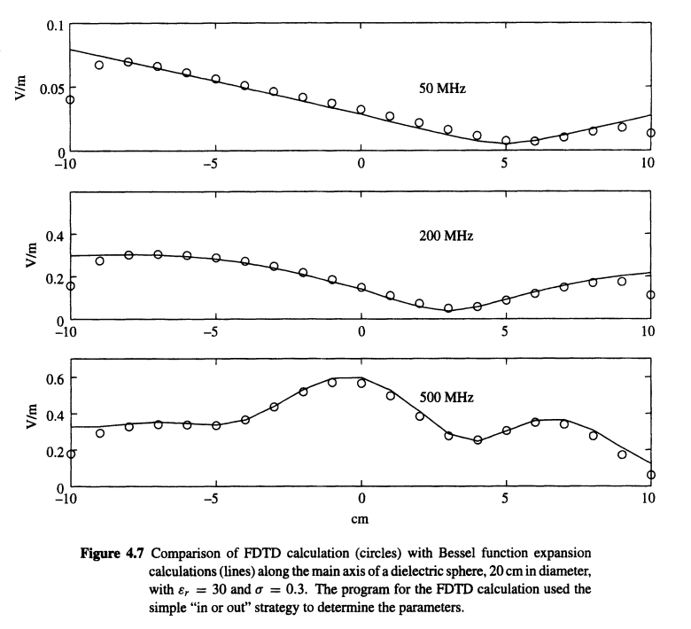
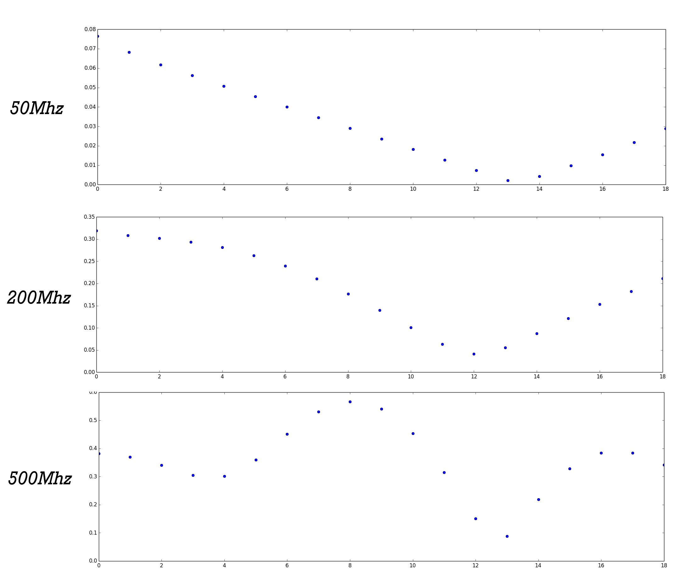
I decided to follow the advice of Sullivan (yet again) and shoot a plane wave at a dielctric sphere and compare the EM energy absorbed by the sphere with analytical results (derived from bessel funciton expansions).

I found very good agreement between his results (left) and mine (right)...
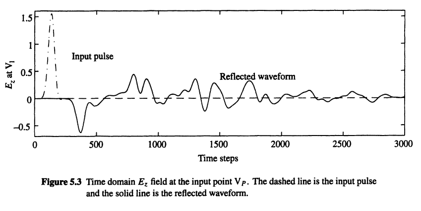
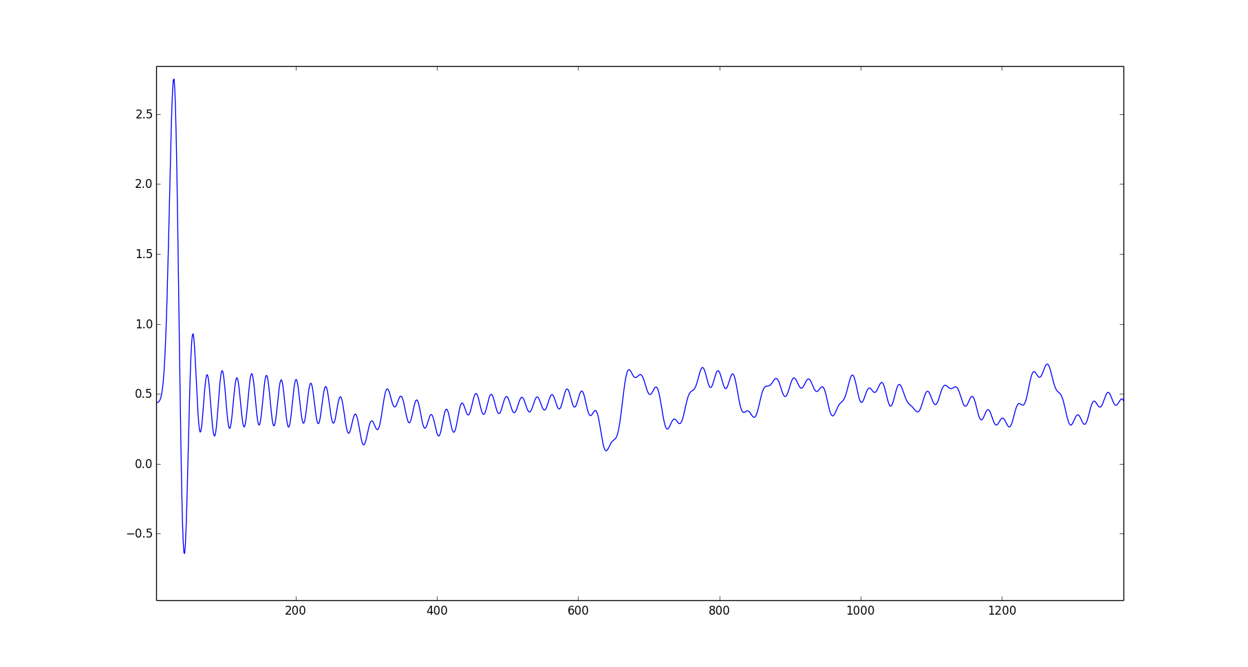
The next measure I tried, was to calculate the transmission/reflection coeffecients of a pulse propogating down a patch antenna.

Unfortunately, I think there is a bug lurking in my code which is causing a significant amount of ripple on my gaussian pulse. This means that there is a lot of added noise and it is hard to evaluate the accuracy of the reflection.
Spiral chip antenna:
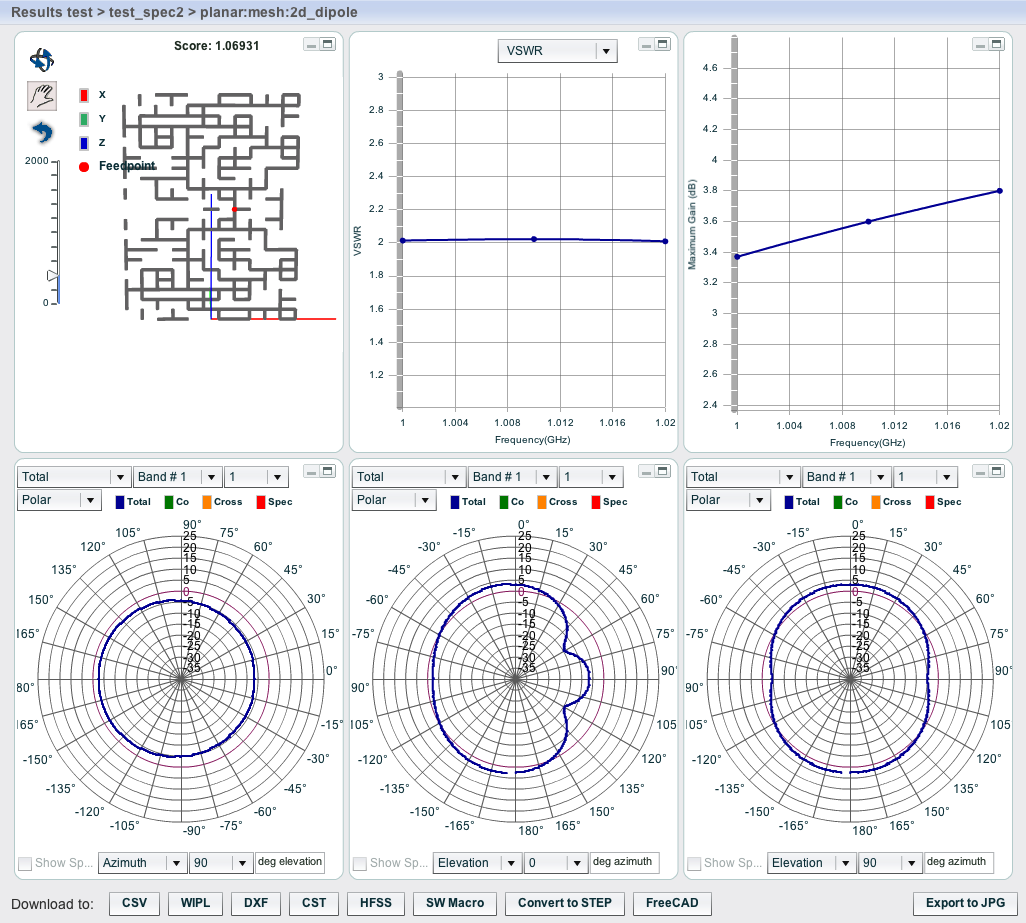
Once all the kinks are worked out, I'd like to try to wrap an optimization around this tool to try to generate designs for discretely assembled electronics and do something similar to what x5systems does for antenna design: