All my code is in this repo, named in honor of the Radon transform’s more eccentric cousin. Building requires a modern C++ compiler and cmake. Libpng must be installed as well. All told it’s about 1,800 lines (excluding third party code), but there’s some unnecessary duplication in there since I’ve been favoring velocity over hygiene.
Let be a density function. If we map density to brightness we can view as describing an image. We’ll assume that this function is defined everywhere, but is always zero outside some finite neighborhood of the origin (say, the bounds of the image).
The projection of to the x axis is obtained by integrating along y:
Meanwhile, the Fourier transform of is
Now comes the key insight. The slice along the axis in frequency space is
So the Fourier transform of the 1d projection is a 1d slice through the 2d Fourier transform of the image. This result is known as the Fourier Slice Theorem, and is the foundation of most reconstruction techniques.
Since the x axis is arbitrary (we can rotate the image however we want), this works for other angles as well:
where is the projection of onto the line that forms an angle with the x axis. In other words, the Fourier transform of the 1D x-ray projection at angle is the slice through the 2D Fourier transform of the image at angle .
Conceptually this tells us everything we need to know about the reconstruction. First we take the 1D Fourier transform of each projection. Then we combine them by arranging them radially. Finally we take the inverse Fourier transform of the resulting 2d function. We’ll end up with the reconstructed image.
It also tells us how to generate the projections, given that we don’t have a 1d x-ray machine. First we take the Fourier transform of the image. Then we extract radial slices from it. Finally we take the inverse Fourier transform of each slice. These are the projections. This will come in handy for generating testing data.
Naturally the clean math of the theory has be modified a bit to make room for reality. In particular, we only have discrete samples of (i.e. pixel values) rather than the full continuous function (which in our current formalism may contain infinite information). This has two important implications.
First, we’ll want our Fourier transforms to be discrete Fourier transforms (DFTs). Luckily the continuous and discrete Fourier transforms are effectively interchangeable, as long as the functions we work with are mostly spatially and bandwidth limited, and we take an appropriate number of appropriately spaced samples. You can read more about these requirements here.
Second, since we combine the DFTs of the projections radially, we’ll end up with samples (of the 2D Fourier transform of our image) on a polar grid rather than a cartesian one. So we’ll have to interpolate. This step is tricky and tends to introduce a lot of error. , but there are better algorithms out there that come closer to the theoretically ideal sinc interpolation. The popular gridrec method is one.
I used FFTW to compute Fourier transforms. It’s written in C and is very fast. I implemented my own polar resampling routine. It uses a Catmull-Rom interpolation kernel.
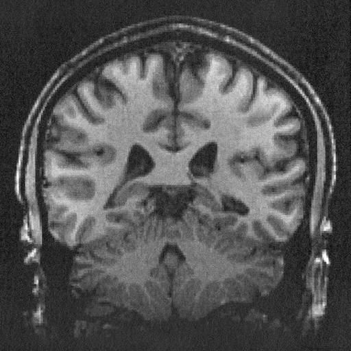
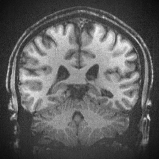
I started with this image of a brain from Wikimedia Commons.
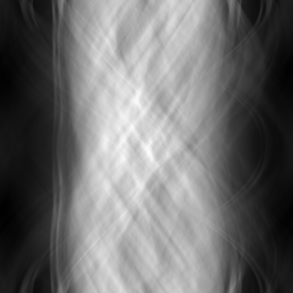
Fourier reconstruction produces a nice sinogram. Each row is one projection, with angle going from 0 at the top to at the bottom, and down the middle column. You can clearly see the skull (a roughly circular feature) unwrapped to a line on the left side of the sinogram.
The reconstruction, however, isn’t so clean.
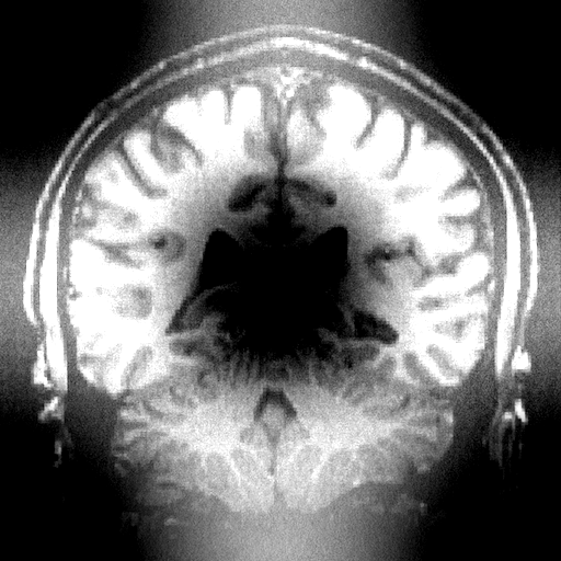
The Fourier library I’m using is solid (and indeed it reproduces images very well even after repeated applications), so the error must be coming from my interpolation code. Indeed, the high frequency content looks ok, but there’s a lot of error in low frequency content. This is encoded in the middle of the Fourier transform, which is what is most distorted by the polar resampling. I could implement a resampling routine specifically designed for polar resampling, or indeed specifically for polar resampling for CT reconstruction, but there are better algorithms out there anyway so I’ll move on.
I got a number of interesting failures before getting my code to work correctly.

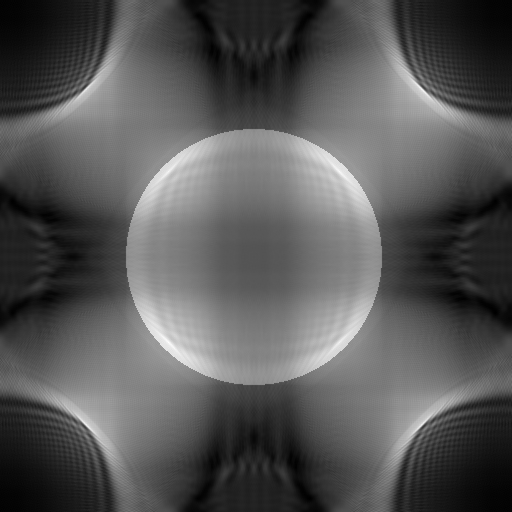
These all started as attempts to project and reconstruct a disk, though I did experiment once interesting mistakes started happening. They mostly result from indexing errors and an issue with my integration with FFTW. The latter problem relates to the periodicity of discrete Fourier transforms and the resulting ambiguity in frequency interpretation. In a nutshell, the DFT doesn’t give you samples of the continuous Fourier transform; it gives you samples of the periodic summation of the continuous Fourier transform. So each sample isn’t representative of one frequency, it’s representative of a whole equivalence class of frequencies.
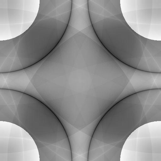
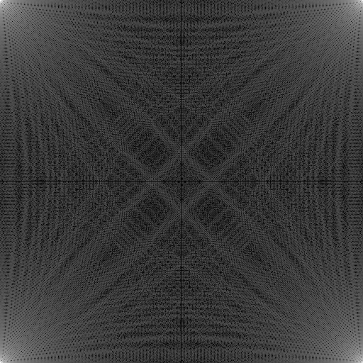
For this application it’s very important that the center of the polar coordinate system used for resampling is right at the DC sample. So though the raw Fourier transform of the image looks like this (real and imaginary parts shown separately),


we want to permute the quadrants so that it looks like this:


Then the center of the image can be the center of the polar coordinate system. (Note: to make these I linearly mapped the full range of each image to [1, e], then applied the natural logarithm. So though they aren’t the same color, both tend toward zero away from the center.) This is akin to viewing the sample frequencies not as , , , , but as , , , , , , .
Interestingly, you can do this by literally swapping quadrants of the image, or by multiplying the results element-wise by a checker board of 1s and -1s. This seems like magic until you just write out the math.
It would be nice if we could avoid the interpolation required for Fourier reconstruction. The simplest way of doing so, and still the most popular method of performing image reconstruction, is called filtered back projection.
Let’s hop back to the continuous theory for a moment. The Fourier reconstruction technique is based on the fact that can be represented in terms of its projections in polar coordinates.
Instead of using interpolation to transform the problem back to cartesian coordinates where we can apply the usual (inverse) DFT, we can directly evaluate the above integral.
To simplify things a bit, note that the integral over is itself a one dimensional inverse Fourier transform. In particular if we define
then the inner integral is just
So overall
Since multiplication in the frequency domain is equivalent to convolution in the spatial domain, is simply a filtered version of . Hence the name filtered back projection.
We’ll replace the continuous Fourier transforms with DFTs as before.
The only remaining integral (i.e. that’s not stuffed inside a Fourier transform) is over , so most quadrature techniques will want samples of the integrand that are evenly spaced in . We want the pixels in our resulting image to lie on a cartesian grid, so our integrand samples should be evenly spaced in and as well.
How do we compute ? We are given samples of on a polar grid. Using the DFT, we can get samples of . They will be for the same values, and evenly spaced frequency values . So if we just multiply by , we get the corresponding samples of . Finally we just take the inverse DFT and we have samples of on a polar grid – namely at the same points we started out with.
This works out perfectly for : we can take the samples we naturally end up with and use them directly for quadrature. For , on the other hand, the regular samples we end up with won’t line up with the values that we want. So we’ll still have to do some interpolation. But now it’s a simple 1D interpolation problem that’s much easier to do without introducing as much error. In particular, we only have to do interpolation in the spatial domain, so errors will only accumulate locally.
I again use FFTW for Fourier transforms. For interpolation I just take the sample to the left of the desired location, and for integration I just use a left Riemann sum. Even with these lazy techniques, the reconstruction looks quite good.
Unfortunately this is still a work in progress. I started implementing a modern approach, but found I didn’t have enough background to make it work. They gloss over some details that I tried to get around with brute force, only to find that the resulting problem was computationally intractable. So yesterday I started over, re-implementing results from one of the original compressed sensing papers. However I did learn some things from my failed attempts…
Both techniques I’ve fully implemented so far involve only three types of operations: DFTs, interpolation, and multiplication (for the filter). All these operations are linear, so we can express them as matrices and reformulate each technique as a single matrix multiplication with a vector. In practice this fact alone is useless, since the resulting matrix ends up being enormous. (In fact if your image and sinogram are n by n pixels, the matrix will have n^4 entries.) But this formulation is used to derive the theory of many total variation versions.
In the process of my first failed total variation implementation, I ended up with most of the parts of the Fourier and filtered back projection algorithms implemented as matrices. So let’s use them and create a sinogram with a single matrix multiplication. As mentioned the matrices are huge, so here I’ll work with a 32 by 32 brain image.

The DFTs were easy. Very similar to the cosine transform we used in the last problem set.


To construct the polar interpolation matrix, I rewrote my interpolation routine to drop the weights it calculated in the appropriate entries in a matrix rather than summing things up as it goes. These weights depend on the type of interpolation used and the sizes of the images involved.

Finally it’s just some (inverse) DFTs to get the sinogram. They can all be expressed simultaneously in one matrix.

I bump up the pixel count for the polar projections so that the resampling doesn’t lose as much information. Thus the final matrix that performs all three of these operations at once has rows and columns, for a total of 8,388,608 entries. (I could chop this in half if I didn’t bother computing the imaginary part of the sinogram. It should be zero but it’s a nice sanity check.)
Ultimately there are a lot more algorithms out there than I care to implement myself. Thanks to the people behind TomoPy, I don’t have to. It’s a library of tomographic imaging algorithms exposed through Python. It’s decently documented, and the code is open source. It also integrates with ASTRA which has some blazing fast GPU implementations.
I scanned a 3d print that I made in How to Make (almost) Anything last semester.
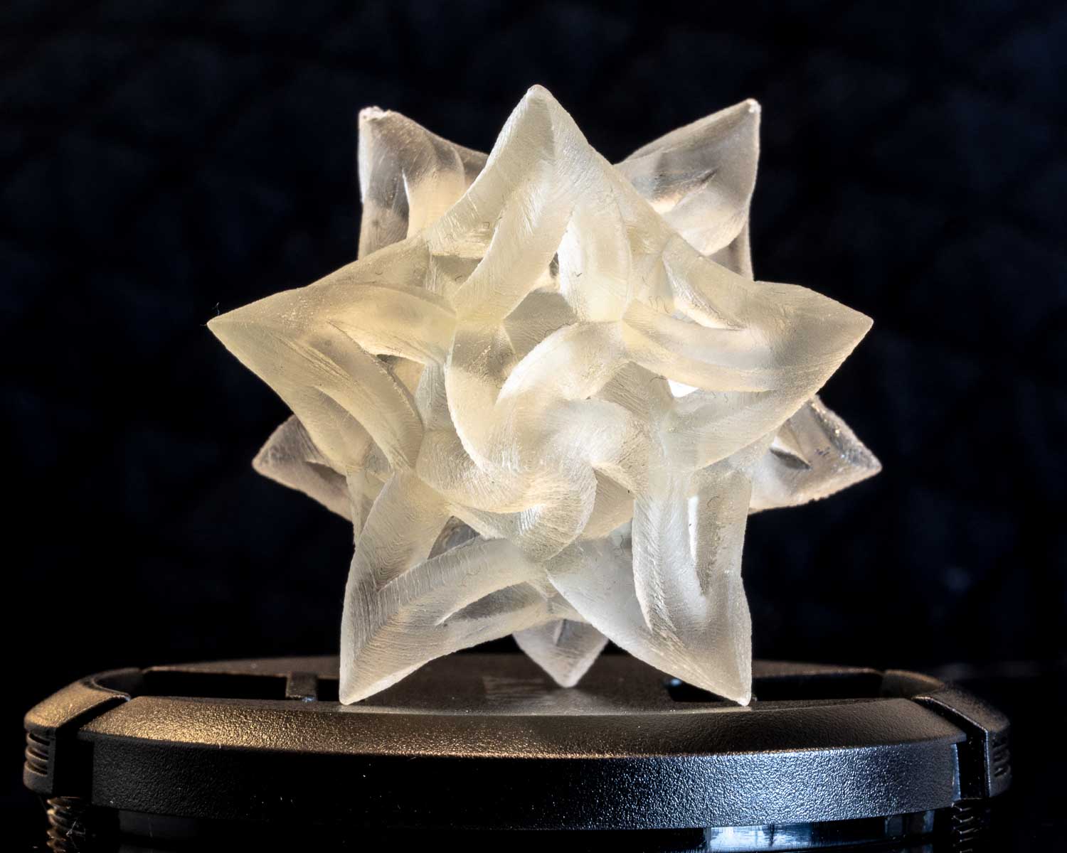
I reconstructed it using TomoPy’s gridrec implementation.
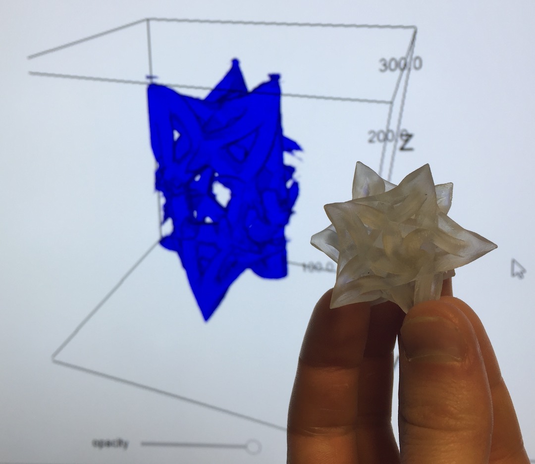
The results aren’t that great, so evidently the settings will require some tweaking. Ultimately I’d like to set up an easy to use TomoPy/ASTRA toolchain to use with CBA’s CT scanner; this is just a first test.
In particular, TomoPy is designed for parallel beam scans, not cone beam scans. In 2D it’s not hard to manipulate fan beam data into a format that parallel beam algorithms can understand, since every line in a fan beam is a line in some other parallel beam. But this doesn’t work in 3D since there’s only one horizontal plane in which the cone beam rays are aligned with the parallel beam rays. Luckily ASTRA supports cone beams, so once I have that integration figured out we should be able to get proper reconstructions.