Week 11 - Interface & Application Programming

This weeks assignments covered applications and interfaces. The individual assignment was write an application that interfaces a user with an input and/or output device. I decided to create an application to visualize the 3D field over time that a 3D hall-effect sensor sees. The sensor was already developed and debugged in Input Devices week. This week constituted communicating the sensor readout with MATLAB which has many tools for visualization, namely a 3D plotter.

The first step of successfully reading to the 3D magnetic field sensor was already accomplished in Input Devices. The following Arduino code was loaded to the centralized SAMD21 uC board.

#include <Tle493d_a2b6.h>
Tle493d_a2b6 Tle493dMagnetic3DSensor = Tle493d_a2b6(Tle493d::FASTMODE,Tle493d::TLE493D_A0);

float TPI = 13; // threads per inch
float DPS = 1.8; // degrees per full step
float FULLROT = 360; //

int currX = 0;
int currY = 0;
int currZ = 0;

int targX;
int targY;
int targZ;

bool hitX = 0;
bool hitY = 0;
bool hitZ = 0;

#define output(pin) (PORT->Group[0].DIRSET.reg = pin)
#define set(pin) (PORT_IOBUS->Group[0].OUTSET.reg = pin)
#define clr(pin) (PORT_IOBUS->Group[0].OUTCLR.reg = pin)
//#define compare(value,pin) (value > pulse) ? set(pin) : clear(pin)

#define Xpos 2
#define Xneg 3
#define Ypos 4
#define Yneg 5
#define Zpos 6
#define Zneg 7
#define LED 11

void setup() {
  Serial.begin(9600);
  while (!Serial);
  
  //If using the MS2Go-Kit: Enable following lines to switch on the sensor
  // ***
  // pinMode(LED2, OUTPUT);
  // digitalWrite(LED2, HIGH);
  // delay(50);
  // ***

  TPI = 13; // threads per inch
  DPS = 1.8; // degrees per full step
  FULLROT = 360; //
  
  currX = 0;
  currY = 0;
  currZ = 0;
  
  targX;
  targY;
  targZ;
  
  hitX = 0;
  hitY = 0;
  hitZ = 0;

  clr(Xpos);
  output(Xpos);
  clr(Xneg);
  output(Xneg);
  clr(Ypos);
  output(Ypos);
  clr(Yneg);
  output(Yneg);
  clr(Zpos);
  output(Zpos);
  clr(Zneg);
  output(Zneg);
  clr(LED);
  output(LED);
//  pinMode(LED,OUTPUT);
//  digitalWriteFast(LED,HIGH);
  
  Tle493dMagnetic3DSensor.begin();
  Tle493dMagnetic3DSensor.enableTemp();

  targX = 4*TPI*FULLROT/DPS;
  targY = 0;
  targZ = 0;
  
}

void loop() {
  if(targX>currX){
    set(Xpos);
    currX += 1;
    hitX = 0;
  }
  else if(targX<currX){
    set(Xneg);
    currX -= 1;
    hitX = 0;
  }
  else{
    hitX = 1;
  }
  if(targY>currY){
    set(Ypos);
    currY += 1;
    hitY = 0;
  }
  else if(targY<currY){
    set(Yneg);
    currY -= 1;
    hitY = 0;
  }
  else{
    hitY = 1;
  }
  if(targZ>currZ){
    set(Zpos);
    currZ += 1;
    hitZ = 0;
  }
  else if(targZ<currZ){
    set(Zneg);
    currZ -= 1;
    hitZ = 0;
  }
  else{
    hitZ = 1;
  }
  
  delay(2);

  if((hitX+hitY+hitZ)<3){
    set(LED);
    Tle493dMagnetic3DSensor.updateData();
    Serial.print(currX*DPS/(TPI*FULLROT),4);
    Serial.print(" ; ");
    Serial.print(currY*DPS/(TPI*FULLROT),4);
    Serial.print(" ; ");
    Serial.print(currZ*DPS/(TPI*FULLROT),4);
    Serial.print(" ; ");
    Serial.print(Tle493dMagnetic3DSensor.getX());
    Serial.print(" ; ");
    Serial.print(Tle493dMagnetic3DSensor.getY());
    Serial.print(" ; ");
    Serial.println(Tle493dMagnetic3DSensor.getZ());
  }
  else{
    clr(LED);
    Serial.println(".");
  }
  
  clr(Xpos);
  clr(Xneg);
  clr(Ypos);
  clr(Yneg);
  clr(Zpos);
  clr(Zneg);
}
									

The code is meant to be in combination with a 3-axis machine and it writes the current positions (X,Y,Z) and the magnetic field reading at the position (Bx,By,Bz) to serial. As long as the application can parse the data written over serial, we can transmit data from the sensor to the uC to a computer running the application.

I chose to work with MATLAB, because I know their plotting and visualization functions pretty well. I also know they have GUI building options for the future (final project) and functions built in to communicate with serial devices. I use the serialport function built into MATLAB to open up a connection to the COM port with my SAMD21.I then readlines and parse the data into the parameters and record them. If I get an error when trying to parse the data into a number, MATLAB has a nice try-catch function that will not stop the program but go to the catch statement instead. This is when it breaks from the continuous readline loop and goes to plotting. On the Arduino side, once the program is done reading the sensor inputs (i.e. is complete probing the domain), it outputs continuous periods. This cannot be converted to a number and therefore triggers the plotting in MATLAB. The MATLAB code is provided below.

clear
clc

device = serialport("COM13",9600);
device.Timeout = 60;
[x,y,z,Bx,By,Bz] = deal([]);

while(1)
    try
        data = char(readline(device));
        RD = str2num(data(1:end-1));
        if(isempty(RD))
            error;
        else
            x = [x RD(1)];
            y = [y RD(2)];
            z = [z RD(3)]; 
            Bx = [Bx RD(4)];
            By = [By RD(5)];
            Bz = [Bz RD(6)];
        end
    catch
        break;
    end
end

figure(1);
plot3(Bx,By,Bz);
xlabel('X (in)');
ylabel('Y (in)');
zlabel('Z (in)');
xlim([-20,20]);
ylim([-20,20]);
zlim([-20,20]);
box on;
grid on;
clear device;
									

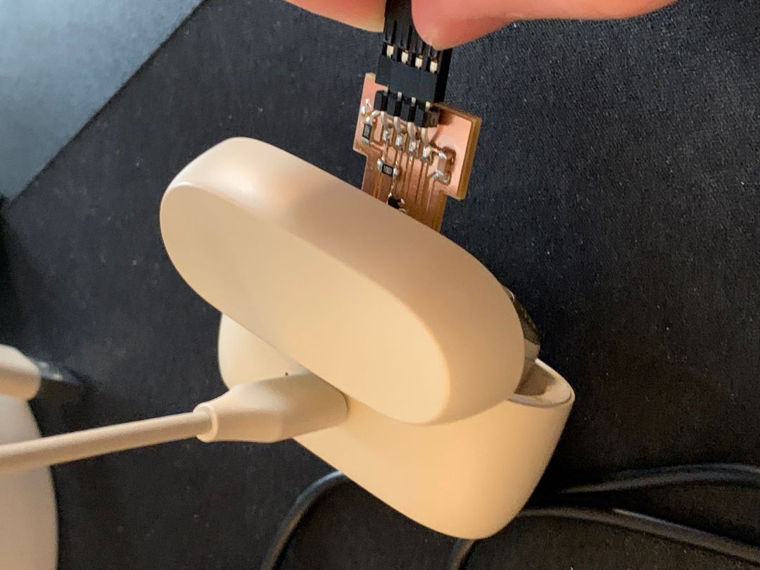
Using the magnet embedded in my wireless earbud charging case, I move it randomly around the sensor during the reading period.

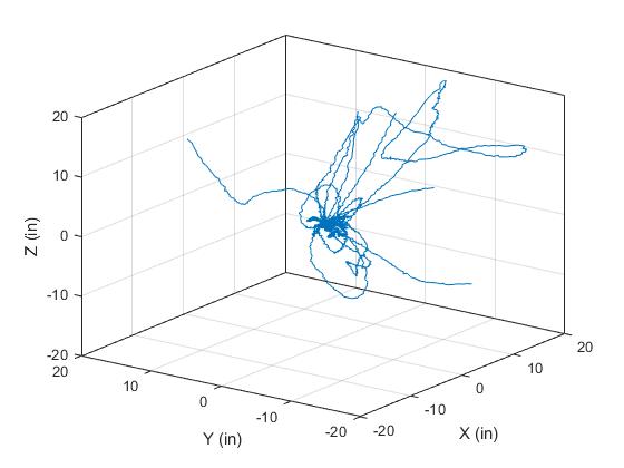
Once the reading period is over, the output looks like below. This shows the path the magnet took in a certain sense, but is actually just 3D magnetic field components plotted. Eventually, this will become a 3D point arrow plot which shows the vector field or a flux density heat map.

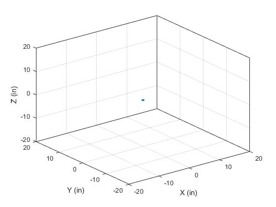
To show that this isn't just gibberish, here is the same plot, without ever bringing the magnet near the sensor. Zero field.

If the field probing and posting to serial is slow enough, the plotting in MATLAB can be done in real time which is my hope eventually. However, if the serial reading happens too frequently the plotting routine in MATLAB can't keep up.

Design files for this week can be found here.