Computing
Boolean Logic
The Transistor
The transistor is the building block of today’s computing technology.
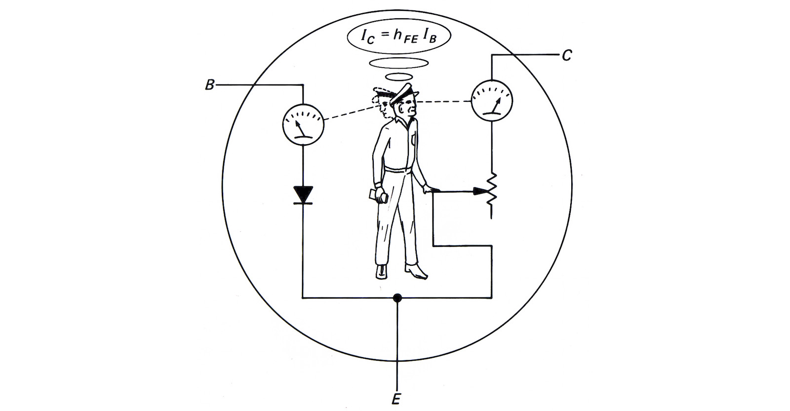 The “transistorman” from the first edition of Horowitz’s The Art of Electronics.
In Claude Shannon’s 1937 master’s thesis (at MIT), he showed that relays could be used to solve Boolean Algebra problems. The rest, as they say, is history.
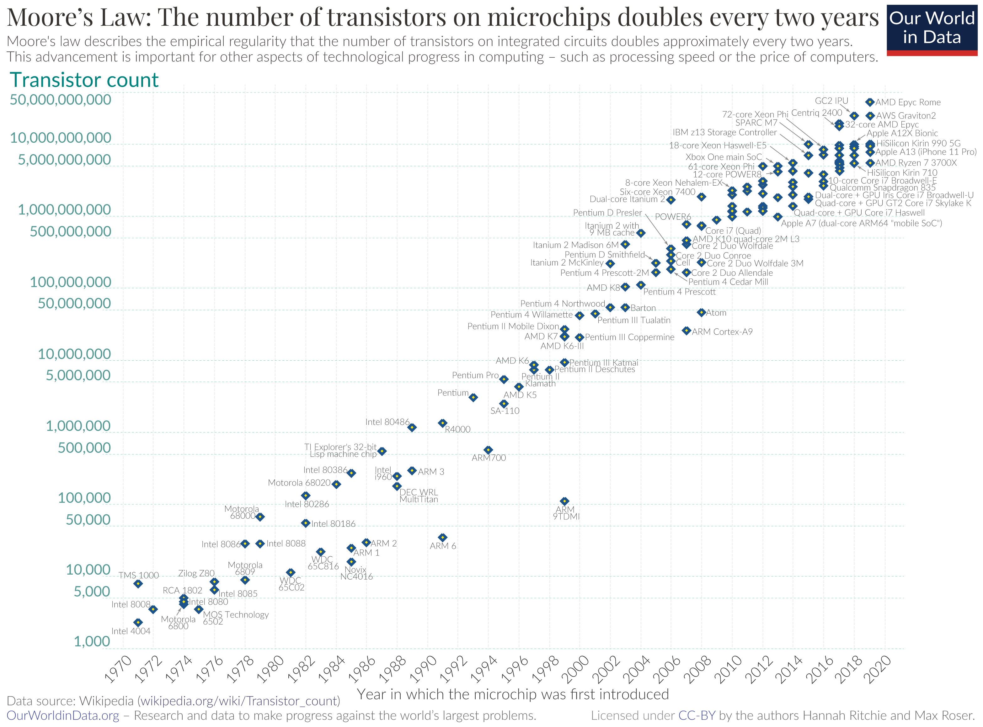 Moore’s Law is dead, long live Moore’s law
Integrated circuits will lead to such wonders as home computers – or at least terminals connected to a central computer – automatic controls for automobiles, and personal portable communications equipment. The electronic wristwatch needs only a display to be feasible today.
– Gordon Moore, 1965
Since the 1970’s the explosion in available computing power has primarily been driven by steady increases in transistor density, most famously codified in Moore’s Law. However, the trend is slowing down. New advances in computing power are increasingly driven by parallelization and/or hardware architecture improvements. Some view this as the beginning of a bleaker era, but others argue there is plenty of room at the top.
PLD
Programmable Logic Devices describes a wide class of logic circuits that can be reconfigured at will (unlike Integrated Circuits) and can provide realtime, asynchronous computations between input signals.
A special type of PLD is the PAL, in which the logical function is implemented as a sum-of-product of the input signals by combining them in AND gates through programmable fuses. The result of several AND gates are then fed through a fixed OR gate.
 source: https://en.wikipedia.org/wiki/Programmable_logic_device
CPLD
A Complex Programmable Logic Devices comprises several PLD that can be connected to one another through a central interconnection matrix, offering more complex combinations.
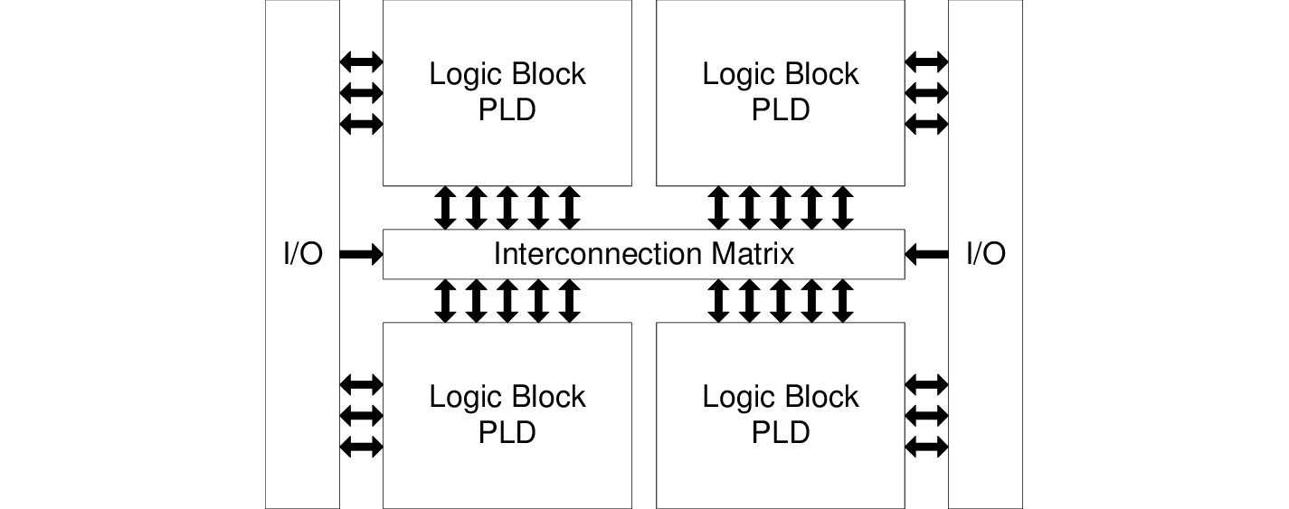 source: Upegui, Andres. (2006). Dynamically reconfigurable bio-inspired hardware. 10.5075/epfl-thesis-3632.
FPGA
Field Programmable Gate Arrays are a type of PLD based on gate arrays. Physically, they consist of a grid of configurable logic blocks (CLBs). CLBs support very complex internal logic. They are usually based predominantly on programmable lookup tables. FPGAs initially grew in popularity since they support simulation of custom logic circuits. Increasingly they are also used for general purpose computing, where extreme speed or power efficiency is required, but it doesn’t make sense to manufacture a full custom chip (which takes a very long time and is very expensive).
They are common in communications equipment, as well as oscilloscopes and logic analyzers. High frequency trading firms use them. They also appear in some consumer electronics devices, like these synthesizers. You can rent enormous FPGAs by the hour on AWS.
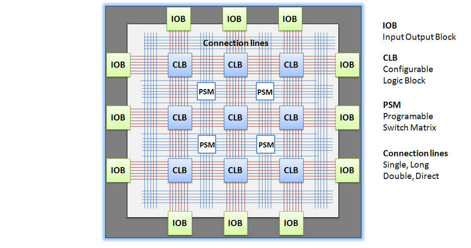 source: http://jjmk.dk/MMMI/PLDs/FPGA/fpga.htm
Embedded Computing
MCU
Microcontrollers are the workhorses of most embedded systems. All microcontrollers have some form of a general purpose computing core and memory. From there there’s a wide array of peripherals, which handle specific tasks at the hardware level. Nearly ubiquitous peripherals include things like general purpose I/O, timers, communications (serial, I2C, SPI, etc.), and interrupts. Some microcontrollers also have hardware random number generators, support for more complex communications protocols (CAN, USB, ethernet), analog electronics components (such as op-amps or instrumentation amplifiers), or additional ways to offload computational work from the main compute core (for example hash/cryptography units or direct memory access).
While the datasheets for many microcontrollers look daunting, once you get the hang of it you learn how to find and digest the small number of pages you have to, instead of getting lost in the 1000s of others. And programming MCUs is usually done in C/C++ (nowadays you can even use Python on some, at the cost of a lot of program memory for the interpreter, and a big hit in performance). So they are among the easiest to use of the embedded devices described on this page.
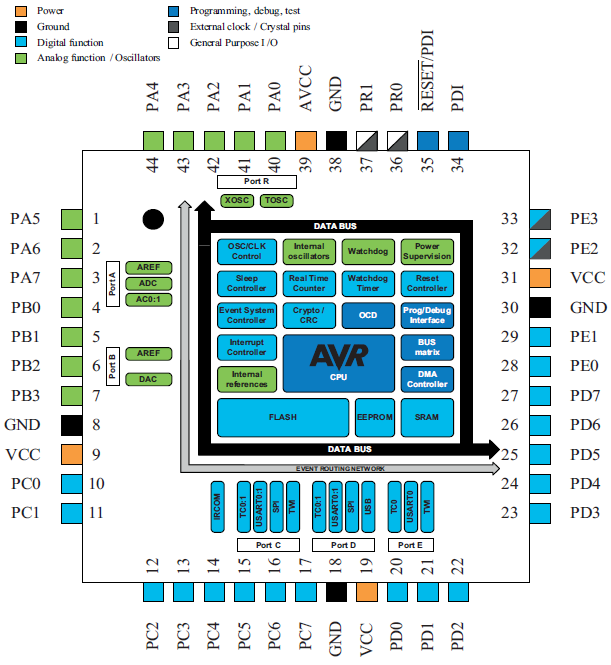 A look inside an XMEGA
Some of CBA’s favorite MCUs include:
- 8-bit AVR MCUs: ATtiny, AVR-DB series
- ATXMEGA series
- ATSAMD11/SAMD21
- ATSAMD51
- NRF52
- STM32
- ESP32
These MCUs support primary clock speeds ranging from a few megahertz to a few hundred megahertz. Main clock speed doesn’t necessarily tell you how fast an MCU will be in sensing and responding to its environment, however, since that involves the speed of the relevant peripherals as well. Measuring ring oscillation rates is a good way to quantify an MCU’s maximum performance when going from bits to atoms and back.
One advantage of the 8-bit AVRs over the powerful 32-bit SAMD family is the simplicity of the peripheral interfacing, with the ability to perform advanced tasks in a single instruction cycle.
A recent development in the peripheral world is the inclusion of some FPGA-like features. Atmel calls this configurable custom logic (see e.g. the ATTINY214). Rasperry Pi calls it programmable I/O (see e.g. the Pico).
Additional resources:
DSP/CODEC
DSPs are specialized microcontrollers for signal processing; they come with the appropriate ADC/DAC and a special set of instructions to handle data transforms with a high vectorization and/or bitrate.
CODECs are essentially just the peripherals from a DSP, tailored for a particular task. For example, the TI PCM2906C can sample a stereo audio signal at 48kHz, and send the data to your computer over USB and play another stereo channel of output. This all happens in hardware; there’s very little coding involved.
MPU
A microprocessor (unit) is just the processing core of an MCU – peripherals not included. Since they lack peripherals, they require additional chips to provide a clock signal, memory, and I/O (at least). However chips marketed as MPUs tend to have more powerful processors than MCUs. They’re also usually intended to run an operating system, unlike most MCUs. The CPU in your computer is a microprocessor, though it probably wasn’t marketed as an “MPU” since that acronym is more commonly used in the embedded systems world.
SoC
A system on a chip is a computing system built around a microprocessor in which all the additional components are soldered onto one board. Raspberry Pis are SoCs, as are BeagleBone Blacks, PCDuinos, etc. Regular Arduinos don’t count since they’re built around MCUs and don’t run any form of operating system. SoCs can be contrasted with motherboard based systems, as found in most PCs, in which the various components are plugged into various sockets instead of soldered down permanently. However many recent laptops are moving in the SoC direction, with soldered RAM etc. This can save cost and potentially produce a faster system (since the manufacturer knows exactly what RAM will be used and can tune the whole system together), but means you can’t slot in an additional stick if you decide you want more memory later, or one of your current chips goes bad.
Personal Computing (PC)
“There is no reason anyone would want a computer in their home.”
– Ken Olsen, founder of DEC, 1977
PCs may seem so common as to not be worth discussing, but now is actually a pretty exciting time in the market.
Today there are two big names in the PC microprocessor market: Intel and AMD. AMD was on the verge of bankruptcy just four years ago, but now their CPUs are beating Intel’s in many benchmarks, and they’re rapidly gaining market share. This has been a wake up call for Intel, and forced them to step up their formerly stagnating innovation game lest AMD eat their lunch.
x86 architecture/CISC
Even as we speak, systems programmers are doing pointer arithmetic so that children and artists can pretend that their x86 chips do not expose an architecture designed by Sauron.
– James Mickens, Professor of Computer Science at Harvard
Intel and AMD have a big similarity, though: both platforms are built on the x86 instruction set architecture. This ISA traces its origins back to the legendary Intel 8086, which was used in the first IBM PC. Since then it’s been extended to 64 bits (originally by Intel’s arch-rival, AMD), and had many additional instructions tacked on. It is unabashedly a complex instruction set computer (CISC) architecture, in that it has a bewildering array of instructions, many of which do a series of very specific things.
ARM/RISC
Reduced instruction set computer (RISC) architectures, on the other hand, offer a smaller number of simpler instructions. If you compile a given program for a RISC architecture and a CISC architecture, the RISC version will tend to have many more instructions to execute. However since RISC instructions are simpler, they often execute faster than CISC instructions. So this doesn’t mean the RISC version will be slower.
RISC architectures tend to be more power efficient than CISC architectures, so unsurprisingly RISC reigns supreme in the mobile market. Most phones use one of the ARM architectures. ARM/RISC is also making headway into the server market. Amazon’s recently developed Graviton processors are ARM. ARM cores are even appearing in the PC market: the M1 chip powering Apple’s newest laptops is also a custom ARM chip. The M1 has a novel architecture that incorporates high efficiency CPU cores, high speed CPU cores, a GPU, and dedicated neural net hardware on a single die, all sharing the same memory space.
Graphics Processing Units
While the CPU offers a complex set of instructions that includes vectorization (MMX, SSE, AVX), there was still a need for a dedicated massive parallelization when dealing with graphical components of OS and videogames. The GPU can be seen as a collection of lightweight CPUs running the same simple program (shader) with varying input parameters. They can store data in both dedicated and shared memory.
GPUs were originally designed for videogames, but there is now a shift towards A.I. computing and realtime simulations, offering viable alternatives to CPU-based supercomputers.
Current status
- NVIDIA
- Turing (2018, e.g. RTX 2080 Ti): tensor cores, raytracing, 4352 shading units
- Ampere (2020, e.g. RTX 3080 Ti): 10240 shading units
- AMD
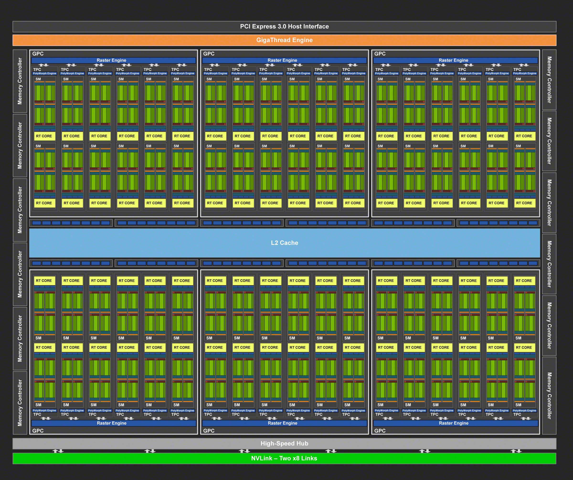 source: NVIDIA
Shaders
Shaders are specialized specialized programs running on the GPU, each with its own task. Object geometry is represented by a set of points, usually linked through edges and faces. The first shaders on the pipeline offer control over this geometry information, while the last shader is responsible for producing color for each pixel (or fragment).
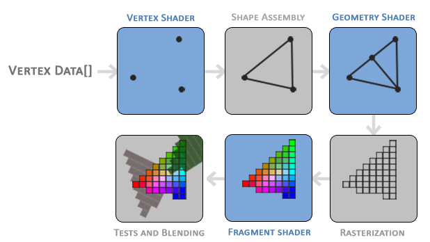
With some advanced trickery, computing can be achieved using shaders. The core idea is to retrieve the result of the computing in the final texture, which is not necessarily displayed thanks to render to texture.
CUDA, OpenCL
Those programming languages offer a more legitimate way of using the GPU for computing, with an elegant API and advanced math libraries. More info on this later.
High Performance Computing (HPC)
Scaling beyond what fits on a single chip or motherboard requires parallelization. So supercomputers are composed of multiple nodes connected by a high speed network. This makes programming a supercomputer very different from programming a regular computer, since the nodes don’t share memory. MPI is the de facto standard for synchronizing and exchanging data between nodes in an HPC system.
Individual nodes function for the most part like powerful PCs, with some exceptions. Today most new supercomputers get most of their FLOPS from GPUs rather than CPUs. So each node will probably have multiple powerful GPUs. NVIDIA V100s are standard today, though the new A100s are faster still and will presumably be common in the next generation. Using GPUs introduces another division of memory, but that’s no different from the difference between RAM and VRAM in any regular computer. Beyond that, it’s now common to see “NUMA nodes”, which stands for non-uniform memory access. This means that certain portions of RAM are physically closer to certain processors, and can be accessed more quickly.
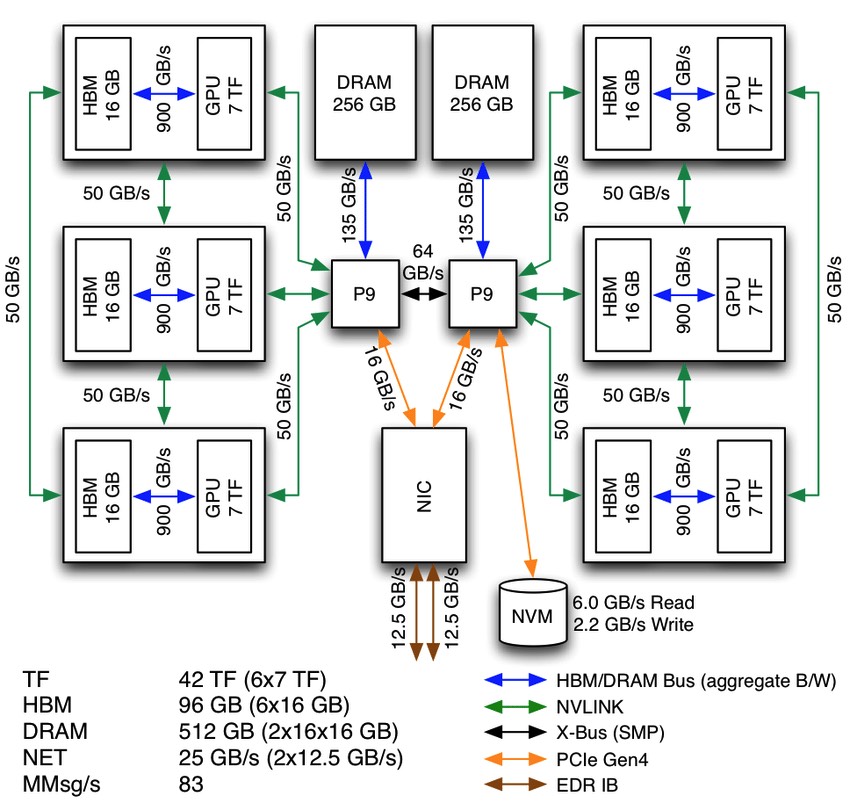 A single node in Summit, showing NUMA architecture
Supercomputers are most commonly measured in peak FLOPS, usually measured on LINPACK or a similar benchmark. Peak FLOPS is traditionally the most important metric, but FLOPS per Watt is becoming increasingly important. Both metrics are tracked and updated closely at top500.org (see Top500 and Green500).
MIT has a new supercomputer called Satori, built in collaboration with IBM. It currently ranks #9 in the world for FLOPS per Watt.
CBA keeps its own table of FLOPS measurements, based on a massively parallel pi calculation. The table currently has entries ranging from Intel 8088 (a variant of the Intel 8086 mentioned above) to Summit, currently the world’s second most powerful computer (in peak FLOPS).
Emerging Computing Technologies
Superconducting Logic
Superconducting Josephson junctions can be used in place of transistors as a switching circuit. Logical circuits made of these elements can be vastly more energy efficient and faster than conventional CMOS circuits. There are two main families: rapid single flux quantum (RSFQ), and adiabatic quantum flux parametrons (AQFP). RSFQ chips can use extremely high clock rates (~100GHz), but require a current proportional to the number of Josephson junctions that can quickly become limiting (though many variants exist which address this in different ways). AQFP chips are ridiculously energy efficient. Like, 24 kbT of energy per junction. Remember that the Boltzmann constant is 1.38 times 10 to the minus 23 J/K. AQFP makes the Landauer limit relevant. Anyway, AQFP is also faster than CMOS, just not RSFQ fast.
Spintronics
Spintronic circuits use magnetics (literally, electron spins) to store information instead of voltages or currents. These circuits can also be vastly more energy efficient than conventional CMOS.
- Two-dimensional spintronics for low-power electronics
- Mutual control of coherent spin waves and magnetic domain walls in a magnonic device
Quantum Computing
Standard CMOS, superconducting logic elements, and spintronics all rely on quantum effects, but they implement regular Boolean logic. Bits are zero or one, never both (well, unless your computer is broken). Quantum computers are a different beast.
Quantum bits, or qubits, exist in a superposition of zero and one. Concretely, this means that when you measure the qubit, there’s some probability that you will see a zero, and some other probability that you will see a 1. In the language of quantum mechanics, each state has an associated complex number, called an amplitude. (Amplitudes are converted to probabilities via the Born rule when measurements are made.) When you have multiple qubits, quantum mechanics requires that you don’t just have amplitudes for zero and one for each qubit independently; you have amplitudes for every possible arrangement of zeros and ones for all qubits. Thus the number of amplitudes grows exponentially with the number of qubits. So with just 10 qubits, a quantum system encodes 210 = 1024 numbers. With 100 qubits, a quantum system encodes ~1030 numbers. 300 qubits gives you more numbers than there are atoms in the universe.
We can’t measure these amplitudes directly, so this isn’t equivalent to having that much data in RAM. But since amplitudes can interfere, you can arrange things so that all the paths to the correct answer interfere constructively, while all the wrong answers have paths that interfere destructively. Then when you make your measurement, you are overwhelmingly likely to see the correct answer. This choreography of interference patterns is what quantum algorithms are all about. Note that this isn’t equivalent to trying all possible solutions in parallel.