Concepts

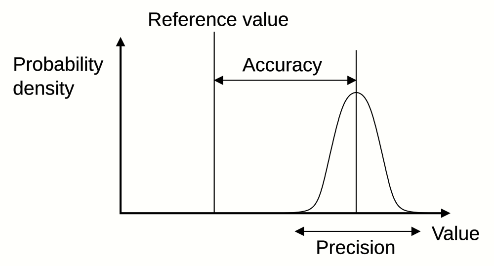
Accuracy and Precision

Accuracy is average error; precision is value consistency. Generally speaking, accuracy is corrected through calibration, but precision is reliant on meausrement technique.

Pekaje at the English-language Wikipedia, GFDL http://www.gnu.org/copyleft/fdl.html, via Wikimedia Commons. Original file here.

Oversampling

Trade bandwidth for resolution, with caveats:

• Each bit costs a factor of 4.
• Requires sensitivity.
• Only increases signal-to-uncorrelated-noise.

Often a built-in ADC peripheral function.

Calibration

Comparison between measured values and a known reference. Zero/span calibration assumes a linear sensor response, and results in slope and offset correction values: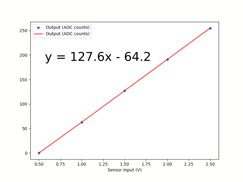

Linearization

If a sensor does not provide a linear electronic response to a stimulus, an added linearization step may be needed. In many cases it’s easiest to implement this as a lookup table with linear extrapolation between points; the size of the table depends on accuracy requirement and available storage: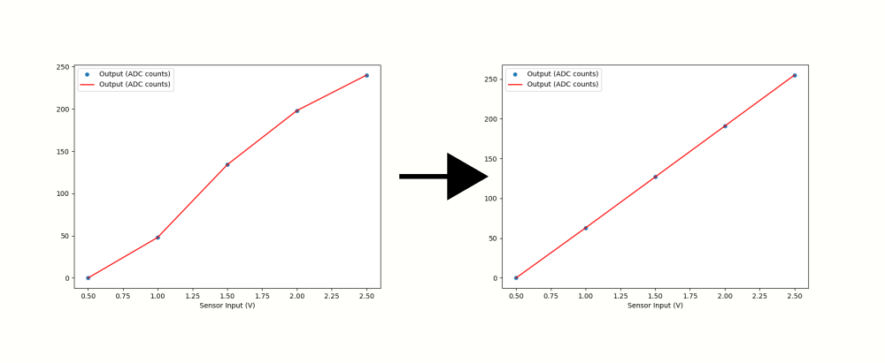

Stability

Sensors drift over time for a veriety of reasons, including component aging, temperature cycling, or inherent lifespan limitations related to the core sensing technology. Stability is often specified in a sensor datasheet in terms of value or percent per unit time; for example, this pressure sensor is advertised to drift less than 0.01 Pa/year.

Turndown

Turndown, or turndown ratio, refers to the practical usable range for a sensor. Generally this means the ratio between the highest measurable value and the lowest within a given accuracy specification. For example, a pressure sensor that can measure up to 1000 psig with 100:1 turndown could be used in an application requiring data down to 10 psig.

Note that turndown is application engineering shorthand; in reality, many sensors will return usable data well beyond their turndown specification, but the resulting value may be unstable or inconsistent device-to-device. When in doubt, test against a standard.

Relative versus Absolute

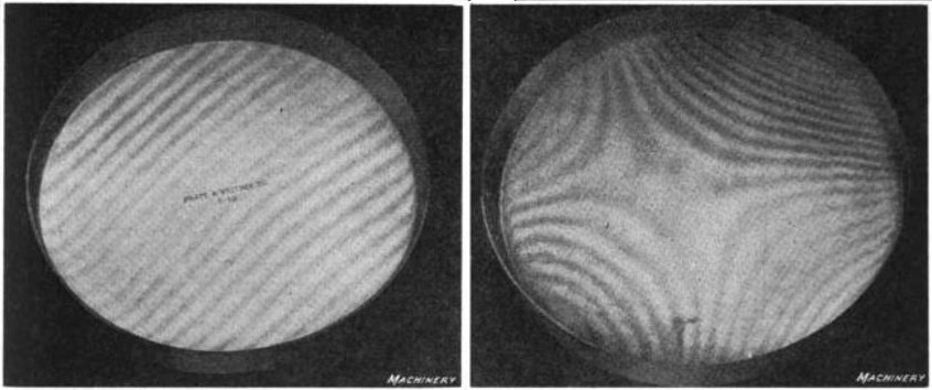Downloaded 2011-03-04 from Franklin D. Jones “How precision gage-blocks are made” in Machinery, Vol. 26, April, 1920, The Industrial Press, New York, p. 706, fig. 21 & 22 on Google Books

Above, an optical flat is used to evaluate the flatness of a piece of glass under monochromatic light. Interference fringes appear whose pattern relates to the relative flatness between the two objects. Comparing two plates of similar flatness won’t tell you which one is off!

Metrology is Relative

Most sensors compare environmental inputs against an internal reference, which then traces its calibration back to a standard. For example:

• a volt meter uses an internal Zener diode-based voltage reference
• a gauge pressure sensor compares an unknown pressure to atmospheric pressure
• a steel rule is created using a printing machine that traces its length calibration back to a standard
• an oscilloscope uses a time standard which is calibrated back to a standard

Eventually, these relative measurements can be traced back a single reference, such as the old kilogram standard, or a fundamental natural constant, such as the resonance frequency of caesium (averaged over a number of atomic clocks).

Turning Physical Phenomena into Electrical Signals

ADCs

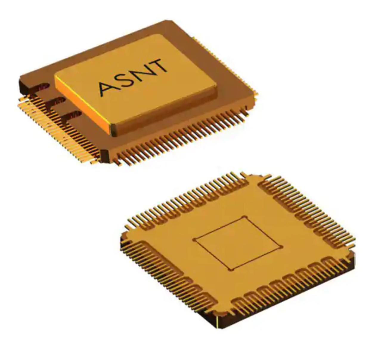
Above, a render of an ADSANTEC 16 GS/s 4-bit flash ADC in a 100-pin metal-ceramic package, yours for only $2400.

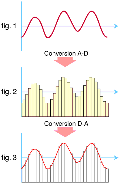
Image credit: Megodenas, Public domain, via Wikimedia Commons: https://commons.wikimedia.org/wiki/File:Conversion_AD_DA.png

Architecture (as seen in the Wikipedia article)

The ADC Tradoff: high speed or high resolution?

• Direct-conversion (“flash”): precision resistor divider network + parallel comparators. Extremely fast; additional bits double required comparators.
• Successive approximation: Comparator + iterative search vs adjusted voltage reference.
• Ramp-compare: Saw-tooth reference waveform compared to incoming signal; comparator fires and checks timer vs waveform.
• Wilkinson: compare input voltage with capacitor charging at a known rate.
• Sigma-delta: converts voltage into pulse frequency:

Pulse-density modulation (blue) vs analog sine wave (red). Image credit: Kaldosh at en.wikipedia, Public domain, via Wikimedia Commons: https://commons.wikimedia.org/wiki/File:Pulse-density_modulation_2_periods.gif

Single-Ended versus Differential

Sampling Rate

Shannon-Nyquist theorem: generally, to fully capture a signal you need to sample at twice its highest frequency component.

Dots on left show sampling points (black) vs reconstructed waveform (orange) and actual signal (grey); pink shading on right shows portion of signal captured as sampling rate increases. Image credit: Jacopo Bertolotti, CC0, via Wikimedia Commons: https://commons.wikimedia.org/wiki/File:Nyquist_sampling.gif

Compressed Sensing: knowledge about signal sparsity = fewer samples than Nyquist to reconstruct.

Exasampler

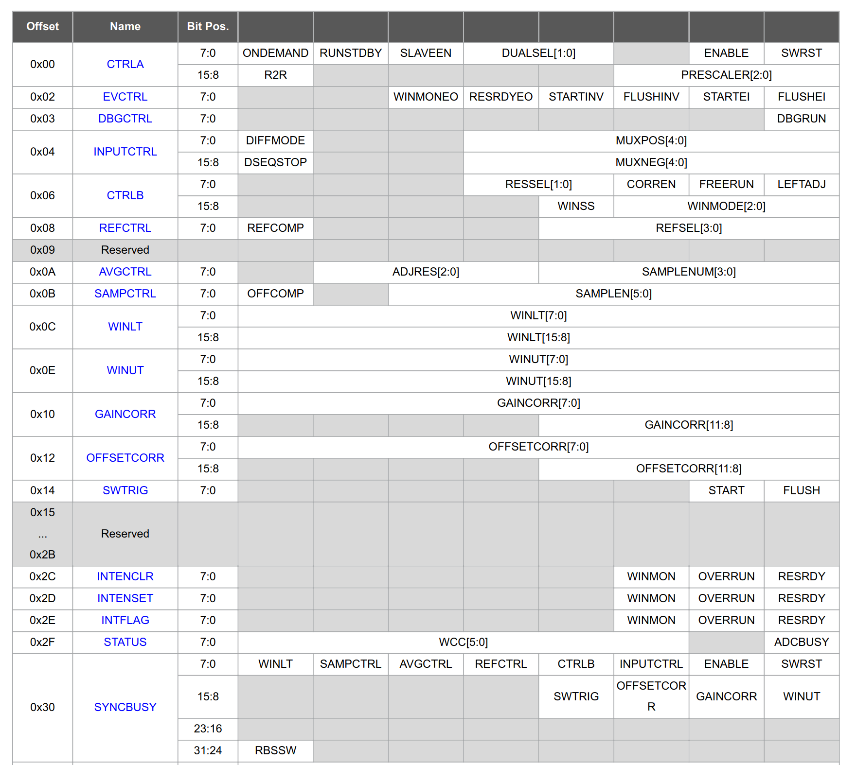
Built-in ADC peripherals vs discrete ADCs

• Discrete for special cases: ultra-high-sensitivity, audio processing, building test equipment, etc.
• Built-in is pretty excellent nowadays
  • SAMD51 ARM Cortex M4F, ~$5
    • 1 Msps (mega-samples per second)
    • 12-bit
    • differential or single-ended
    • 32 inputs (but you can’t do 1 Msps simultaneously on all of them)
    • Built-in oversampling to 16-bit
  • AVR128DB32, ~$2
    • 130 ksps (kilo-samples per second)
    • 12-bit
    • differential or single-ended
    • 22 inputs (but you can’t do 130 ksps simultaneously on all of them)
    • connected internally to OPAMP peripheral: PGA, instrumentation amp, etc.

AnalogRead() vs:

Filtering

Kalman filtering: joint probability distribution across variables; recursive; assumes data normality. Example: sensor fusion from an IMU, using magnetometer, accelerometer, and gyroscope data to estimate position.

Particle filtering: Monte Carlo method, plus math