Optimal Control Theory

Prerequisites:

• ODEs
  • dynamic model that relates the inputs to the outputs: empirical, differential eqns
  • review from Nature of Mathematical Modeling and Neil’s book: HERE
• Linear Algebra
  • eigenvalues & stability
  • Gilbert Strang, MIT Open Courses

Dynamic Model: The Inverted Pendulum

The derivations of the equations of motion (Lagrangian Mechanics) for this system are described HERE.

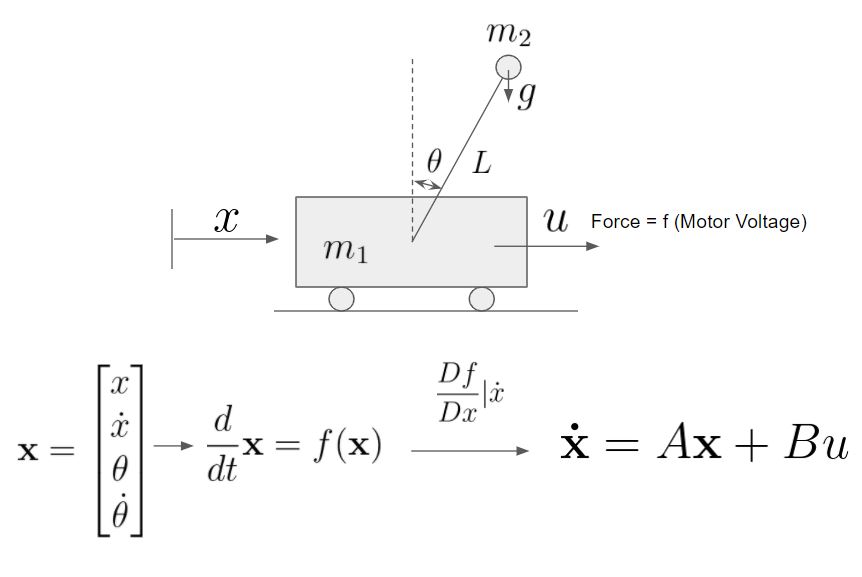
Integrating the equations of motions for the system allows us to understand the dynamics of the system and start thinking about the control strategy to achieve stabilization:

Eigenvalues & Stability

The eigenvalues and eigenvectors of the system determine the relationship between the individual system state variables (the members of the x vector), the response of the system to inputs, and the stability of the system.

Here is a video to understand mathematically the relationship of eigenvalues and stability.

• if all eigenvalues negative -> system is stable
• the goal is to add actuation (Bu to Ax) to force eigenvalues to become positive and thus achieve system stability

Controllability

• Can I steer the system anywhere given some u?

• controllability: ctrb(A,B) is a number that if it is equal to the number of states ( spans the state space), then the system under examination is controllable

Here is a video to understand the math involved if you want to demonstrate observability.

Linear Quadratic Regulator (LQR)

• So, we know that we can simulate the inverted pendulum on a cart, the full nonlinear system without control.

• Also, we know that we can linearize about the fixed point where the pendulums up to get an a matrix and a D matrix

• We know that the system is in fact controllable so if we look at the rank of the controllability matrix it has dimension 4 so it spans the four dimensional state space of the position and velocity of both the carts and the pendulum

• Lastly, we know that since the system is controllable we can design a full state feedback u equals minus KX so that I can place the eigenvalues of the closed-loop system anywhere I want okay and it’s one line in MATLAB where you specify the eigenvalues and it will find this gain matrix K - to move your system to those eigenvalues we then take that control law apply it to the full nonlinear system and we show that in fact we can stabilize this up unstable inverted pendulum configuration.

Full-State Estimation

In real life, we don’t actually often have access to my full state measurements of my system so for example on the inverted pendulum on a cart maybe I don’t want to measure all four of my state variables maybe I just want to have an encoder to measure the theta position and then I ask myself the question can I back out the full state?

• observability: obsv(A,C)
• Can I estimate any state x from a time series measurements y(t)?

so what we’re going to be doing is we’re going to not only develop a controller we’re also going to develop something
called an observer or an estimator so that given Y we’re going to back out what X is and we’re going to use that as a proxy for this linear quadratic regulator

So in a more realistic system:

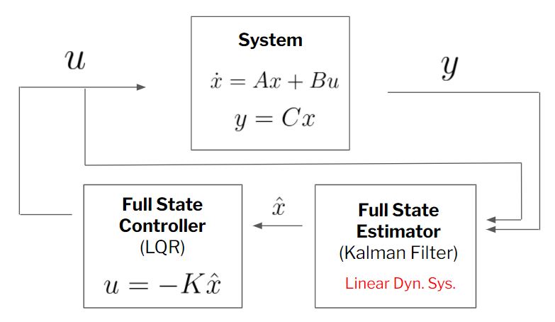
we can apply the notions of controllability with matrices A and B now we’re and observability with matrices A and C to ask the following question: if a system is observable can we build an estimator so that only given measurements of Y we can reconstruct what the full state of the system is for use with full state feedback control?

Observability

Here is a video to understand the math involved if you want to demonstrate observability.

Estimators & the Kalman Filter: An Optimal Full-State Estimator

ready to build the common filter okay so the common filter is basically the analog of the linear quadratic regulator for estimation it’s the optimal full state estimator given some knowledge about the types and magnitude of disturbances and measurement noise that I’m going to experience

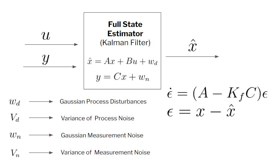
Simple biasing, Kalman filters, and Moving Horizon Estimation (MHE) are all approaches to align dynamic data with model predictions. Each method has particular advantages and disadvantages with a main trade-off being algorithmic complexity versus quality of the solution.

Kalman filtering produces estimates of variables and parameters from data and Bayesian model predictions. The data may include inaccuracies such as noise (random fluctuations), outliers, or other inaccuracies. The Kalman filter is a recursive algorithm where additional measurements are used to update states (x) and an uncertainty description as a covariance matrix (P).

The extended Kalman filter (EKF) is the same as the Kalman filter but in applications that have a nonlinear model. The model is relinearized at every new prediction step to extend the linear methods for nonlinear cases. The unscented Kalman filter (UKF) shows improved performance for systems that are highly nonlinear or have non-uniform probability distributions for the estimates. UKF uses sigma points (sample points that are selected to represent the uncertainty of the states) that are propagated forward in time with the use of simulation. Points that are closest to the measured values are retained while points that are beyond a tolerance value are removed. Additional sigma points are added at each sampling instance to maintain a population of points that represent a collection of potential state values.

Biasing is a method to adjust output values with either an additive or multiplicative term. The additive or multiplicative bias is increased or decreased depending on the current difference between model prediction and measured value. This is the most basic form of model updates and it is prevalent in industrial base control and advanced control applications.

Moving horizon estimation (MHE) is an optimization approach for predicting states and parameters. Model predictions are matched to a horizon of prior measurements by adjusting parameters and the initial conditions of the model.

Model Predictive Control (MPC)

https://www.youtube.com/watch?v=YwodGM2eoy4&list=PLMrJAkhIeNNR20Mz-VpzgfQs5zrYi085m&index=47

Model Predictive Control (MPC) is a powerful optimization strategy for feedback control. The principle behind MPC is the following: if you have a model of your system of interest, you run forward in time a set of forecasts of this model for different actuation strategies and then you optimize over the control input (u) over a short time period. In this way, essentially you determine your immediate next control action based on that optimization. Once you’ve applied that immediate next control action, then you re-initialize your optimization over, you move your window over, you re-optimized to find your next control inputs and this thing essentially keeps marching that window forward and forward in time.

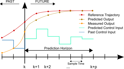
A method to solve dynamic control problems is by numerically integrating the dynamic model at discrete time intervals, much like measuring a physical system at particular time points. The numerical solution is compared to a desired trajectory and the difference is minimized by adjustable parameters in the model that may change at every time step. The first control action is taken and then the entire process is repeated at the next time instance. The process is repeated because objective targets may change or updated measurements may have adjusted parameter or state estimates.

Model predictive control could have multiple input or manipulated variable (MV) and output or controlled variable (CV) tuning constants. The tuning constants are terms in the optimization objective function that can be adjusted to achieve a desired application performance.

Why MPC over PID?

• multiple MVs and MCs
• different number of MVs and MCs

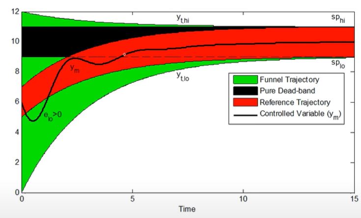
• Target Trajectories
  • Funnel Trajectory
  • Pure dead-band
  • Reference Trajectory
• Response Target
• Response Speed
• Near-term vs Long-term objectives

Pendulum Stabilization Control Examples

• Optimization Library used: LINK

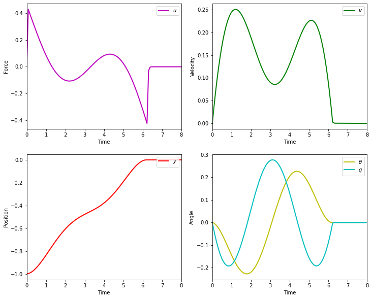
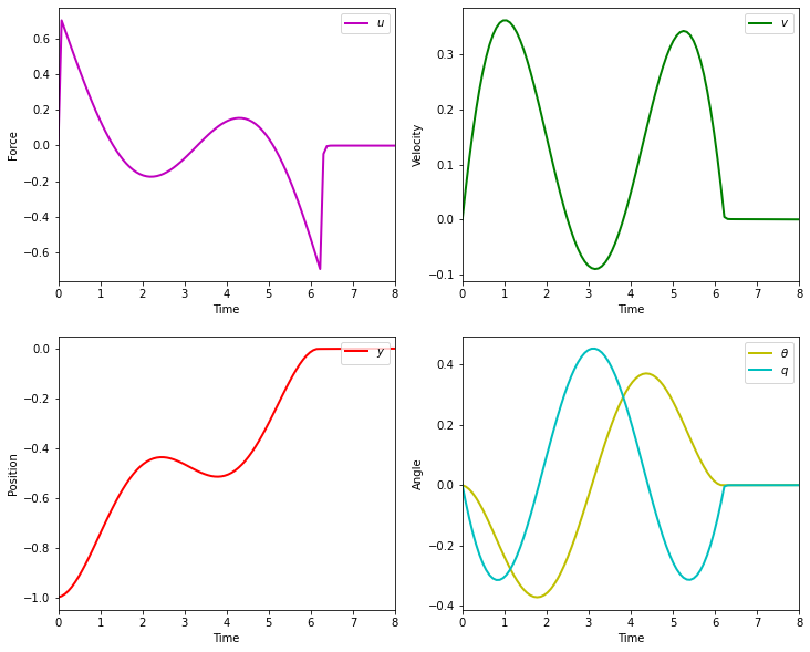
The objective of the controller is to adjust the force on the cart using the state space model in order to move the pendulum from one position to a new final position within a specified amount of time and with minimum force and oscillations at the final position. We need to ensure that the initial and final velocities and angles of the pendulum are zero. The position of the pendulum mass is initially at -1 and it is desired to move it to the new position of 0 within ~7 seconds. Our goal is to design a controller that tunes the actuation force u such as that with changes in the pendulum position the final pendulum mass arrives and remains at the final position without oscillation.

• m2 = 1

• m2 = 8

• m2 = 20

Inverted Pendulum

• m2 = 1

• m2 = 20

• control weights