Reinforcement Learning

Reinforcement Learning is a field closely related to control theory. Its formalism is a little different, and its techniques are traditionally associated with machine learning. These days it’s dominated by the use of deep neural networks. As data driven control theory merges more with machine learning, the boundary between these two fields is blurring.

Markov Decision Processes

A MDP formalizes an agent acting and reacting within some larger system. The model is based on a graph of states rather than a system of differential equations. Specifically, the world of a MDP is modeled as a set of states. In each state, there is a possible set of actions that can be taken. The agent selects one of these, and in response the system moves into a new state. This state change is a random process, but the distribution of next possible states can depend on the previous state and the action that the agent takes. Each state transition is associated with a reward (or penalty). The goal of the learning algorithms below is to choose actions that maximize the expected future reward (often with some form of time discounting applied).

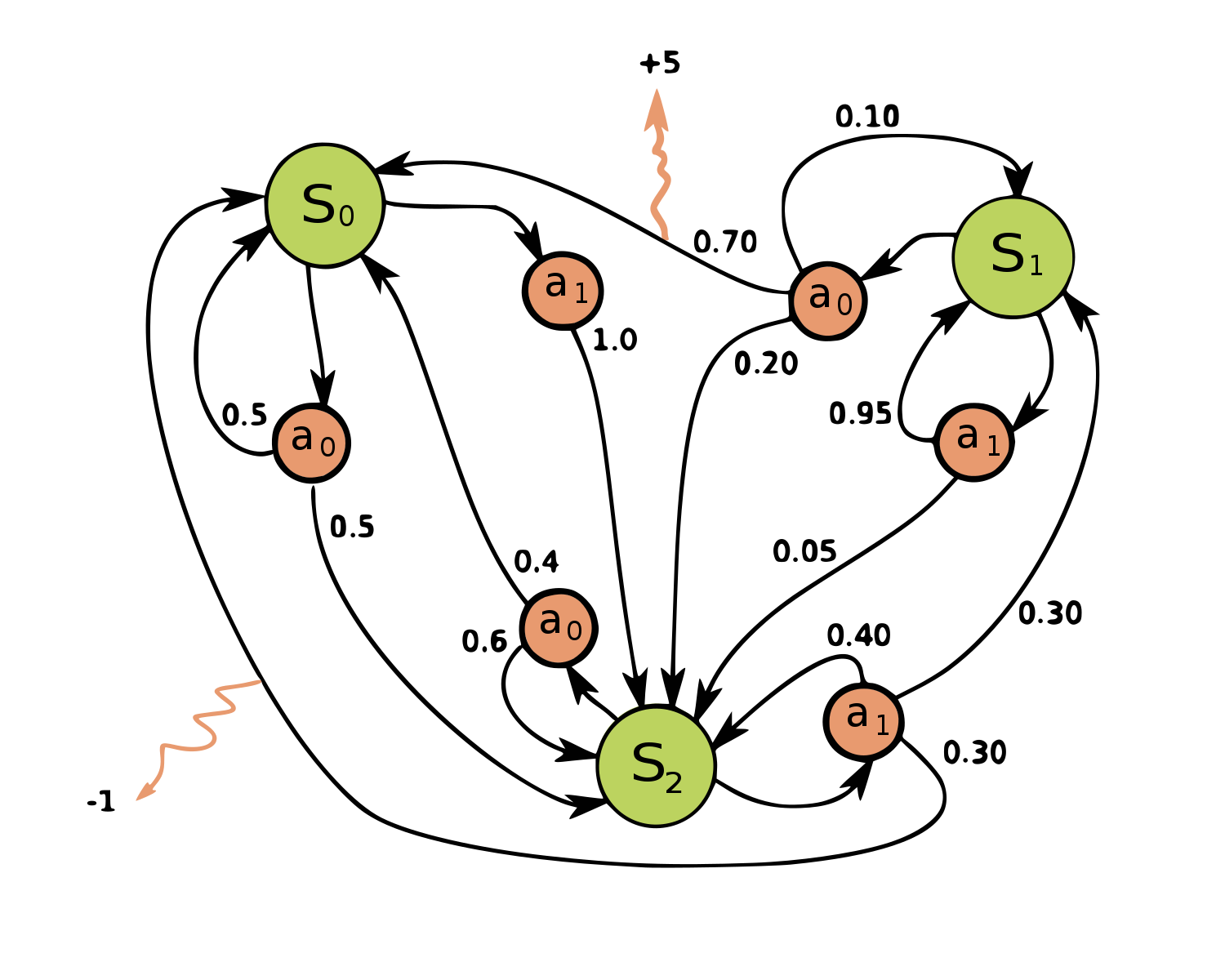Source: https://en.wikipedia.org/wiki/File:Markov_Decision_Process.svg

A policy, in the context of reinforcement learning, is a probability distribution over the possible actions for each state. If the policy is deterministic, then a single action for each state will have probability 1 (and all other actions for that state, probability 0). But this certainly isn’t required. All reinforcement learning algorithms are ultimately trying to come up with the policy that maximizes the cumulative future reward.

Q Learning

Q learning is a model free reinforcement learning algorithm. It is named after the “quality function” at the heart of the method (and has nothing to do with the deep state or certain members of Congress). In particular, the Q function tells you what the total expected future reward is for choosing an action \(A\) in a state \(S\), assuming the best possible actions are chosen from there on out. If you knew this function, writing a policy would be easy: always choose the action with the highest expected reward. Sounds too good to be true, and of course we can’t assume a way to compute it a priori. But the interesting thing is that if we initialize a lookup table of Q values with random numbers, there’s a procedure we can use to iteratively improve it until we get arbitrarily close to the real values. The key insight is that q values of successive states are related: if choosing action \(a_i\) in state \(s_i\) leads us to state \(s_{i+1}\) and gives us a reward \(r_i\), then the following holds.

\[Q(s_i, a_i) = r_i + \max_{a_{i+1}} Q(s_{i+1}, a_{i+1})\]

The \(\max\) is taken over possible actions for state \(s_{i+1}\). It’s how we bake in the notion of choosing the best actions in the future. Technically speaking, it’s only an exact equality if the process isn’t stochastic. Otherwise, perhaps we got unlucky with what state we ended up in, and the real expected reward is higher; or we got lucky and the real expected reward is lower. But if we throw in a learning rate and just push our estimated Q values in the direction suggested by this equation, it turns out that the numbers still converge to the correct values even for stochastic processes (under some assumptions on the learning rate and MDP distributions).

In modern usage, the Q function is usually estimated by a deep neural network. This is the algorithm that first put DeepMind on the map (back before Google owned them) by learning to play Atari games (video).

As another example, several years ago I trained a deep Q learning network to play a game inspired by CNC milling. The algorithm is given a target shape, and the current workpiece shape. At each time step it chooses a direction to move, and if it moves into a pixel occupied by the workpiece, that material is removed. If it moves into a pixel that’s part of the target shape, that’s a mistake and it loses. It solved small problems perfectly. One of these days I still want to get around to scaling it up.

Policy Gradients

With Q learning, once our estimated Q values start to converge, we can easily express our policy in terms of them. Policy gradient methods take a more direct approach, and seek to optimize a policy directly. As with Q learning, these days the policy is almost always represented by a deep net, and we want to train this network with some form of gradient descent.

The first tricky part is that we want to maximize the reward we receive, but we don’t know exactly what the reward function is. We just get samples from it when we perform actions. We certainly can’t compute the gradient of the reward function with respect to the parameters of our neural net. So how can we use gradient descent?

It turns out that since we’re optimizing an expected value instead of a single value, we don’t actually need to differentiate through the reward function at all. We just need to differentiate through the policy, which is exactly what backpropagation on our neural network gives us. The math works out like this. Here you can take \(f(x)\) to be the cumulative total reward for some arbitrarily long amount of time, or as is often the case, the cumulative reward when the game ends. Similarly, \(p_\theta(x)\) should be viewed as the probability of the whole series of actions that got us to that particular cumulative reward. \(\theta\) holds whatever we use to parametrize our policy network, so in practice the weights and biases in our neural net.

\[\begin{aligned} \nabla_\theta \mathbb{E}_{p_\theta}[f(x)] &= \nabla_\theta \sum_x p_\theta(x) f(x) \\ &= \sum_x \nabla_\theta [p_\theta(x) f(x)] \\ &= \sum_x \frac{\nabla_\theta p_\theta(x)}{p_\theta(x)} p_\theta(x) f(x) \\ &= \sum_x \nabla_\theta [ \ln p_\theta(x) ] p_\theta(x) f(x) \\ &= \mathbb{E}_{p_\theta}[f(x) \nabla_\theta \ln p_\theta(x)] \end{aligned}\]

The second tricky thing is that, in the expression above, \(p_\theta(x)\) represents the probability of the whole chain of actions that gets us to a final cumulative reward. But our neural net just computes the probability for one action. This is where the Markov property comes into play. It means that the probability of ending up in some state depends only on the previous state and the chosen action – there’s no dependence on deeper history. So the probability of the whole chain of actions factors into the product of the probabilities of each individual choice we made.

The key parts of this algorithm were first put together in the REINFORCE algorithm. Since then they’ve been expanded on and improved, including ways to reduce the variance of the gradient estimators, deal with black box functions in the policy computation that you do want to differentiate through, and integrating these principles into other algorithms like Monte Carlo tree search. The most famous example of the latter (policy gradients and MCTS) is AlphaZero, which is a general algorithm that can now train itself from scratch to become the best in the world at at chess, go, and many other games without using any historical data. This blog post has a good introduction to AlphaZero, or you can read the full paper.