Optimization

Since so much of control theory relies on optimization techniques, we review some of the most popular methods here.

Gradient Free Methods

The methods in this section only need to be able to evaluate the objective function. No derivatives required. This makes them easily applicable to a wide variety of systems, including those where derivatives are difficult or computationally expensive to compute. However when derivatives are readily available, these techniques will tend to converge more slowly than gradient based methods.

Nelder-Mead

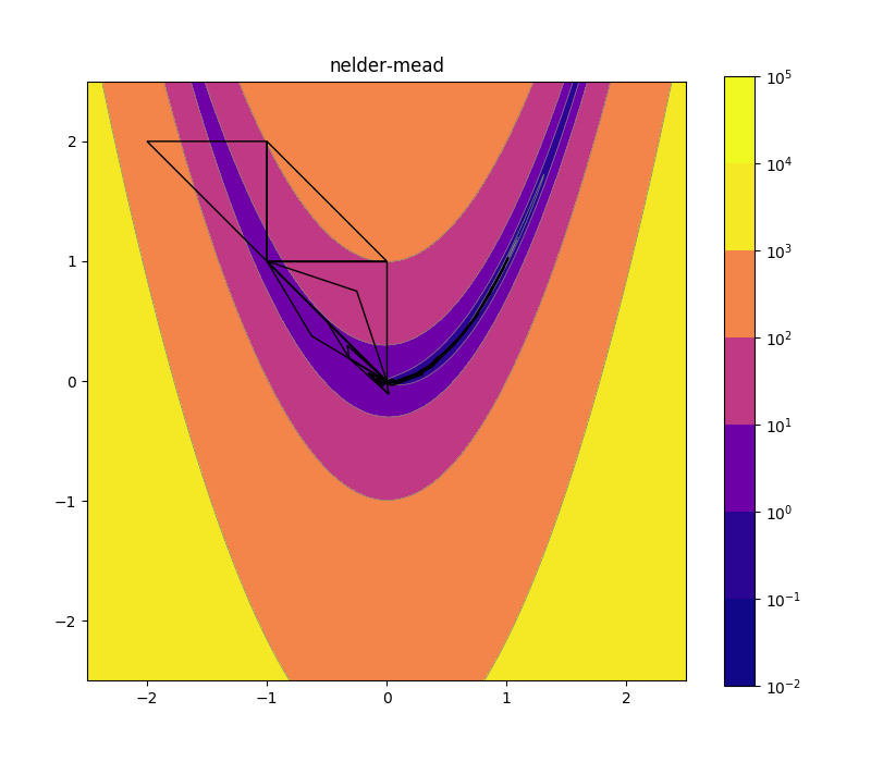
Nelder mead is a heuristic search algorithm with a simple geometric interpretation. You’ll also see it called the simplex method.

In two dimensions, the current search state is encoded as a triangle. In each iteration, we try to move the highest of the three points to a better (i.e. lower objective value) location. The default move is to flip the highest point across the line segment defined by the other two points. There are also moves that expand or contract the area of the triangle as needed (so it can shrink to squeeze through narrow valleys, or expand to quickly march across wide plateaus). In higher dimensions, we use a simplex instead of a triangle, but the same principles apply.

Nelder-Mead tends to work wonderfully up to a dozen or so dimensions, and then quickly becomes quite inefficient. But for low dimensional problems it’s a great first choice since it’s extremely simple and often quite robust.

Simulated Annealing

Simulated Annealing is inspired by metallurgical annealing. At each step it chooses a random direction and moves some distance forward. If the result is better than the last point, the move is accepted. If it’s not better, with some probability the move is still accepted; otherwise, another direction is considered. The probability of accepting bad moves decreases over time. The insight is that it might be necessary to climb over a ridge in order to get to a lower valley. So though simulated annealing isn’t guaranteed to find a global as opposed to local optimum, depending on the objective function and the annealing schedule (how the probability of accepting bad steps changes over time), it can be quite effective at this in practice.

CMA-ES (Genetic Algorithms)

CMA-ES stands for covariance matrix adaptation evolutionary strategy. Its search state is encoded as a multivariate Gaussian distribution. It draws samples from this distribution, evaluates the objective function at them, and based on the resulting values updates the distribution such as to increase the probability of drawing better samples. The basic idea behind the update mechanism is that the worst samples in each round are discarded, and the rest are used to compute a new mean and covariance matrix. The actual math gets a lot more complicated than that, unfortunately, so unlike Nelder-Mead or simulated annealing, this is a tricky algorithm to implement yourself.

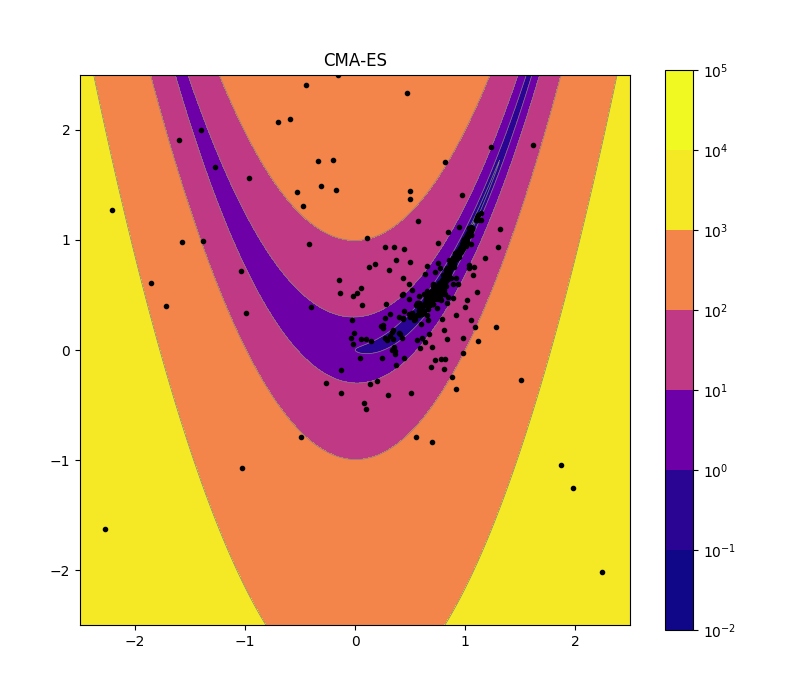
CMA-ES is a particularly sophisticated example of a broader class of optimization techniques known as genetic algorithms. Genetic algorithms are loosely modeled after biological evolution. So each sample point has to have a “genome” that can be combined with others to produce a new sample, and the objective function acts as the fitness function. The challenge is that finding suitable analogs of crossover, mutation, etc. is often very challenging. So without a reasonable intuition for how subparts of a solution can be productively combined, it can be difficult to get started. CMA-ES gets around this by using statistically sound update rules for a distribution, stepping back from the more literal biological analogies.

Particle Swarm Optimization

Particle swarm optimization is similar to CMA-ES, but instead of drawing samples from some distribution, each sample moves around somewhat independently. Samples are treated as particles with position and momentum. They move downhill based on local information (their recent evaluations), but also on some shared knowledge about the best solutions found so far by any other particles.

Gradient Based Methods

When applicable, gradient based methods can converge much faster than gradient free methods.

Gradient Descent

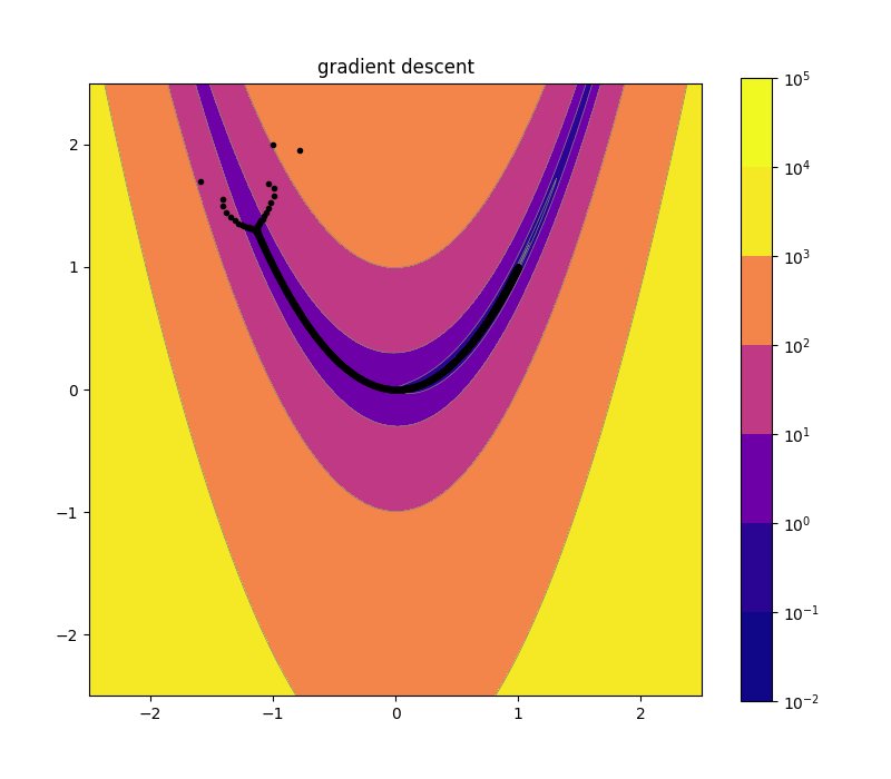
The idea behind gradient descent is simple: always move downhill. In the simplest version, in each iteration you simply take some fixed size step in the downhill direction. Often the step size is decreased over time (similar to how the annealing schedule is used in simulated annealing). More sophisticated versions rely on a line search, which just means moving in that direction until you start going uphill again. This ensures you move as far downhill as you can in each step, but it also has a major drawback: you also end up taking 90 degree turns at each step. This means that this version of gradient descent can be very slow to move along narrow valleys, since it has to zig zag along instead of moving in a straight line. You can see this in the upper left portion of the image below, where the algorithm started.

Stochastic Gradient Descent

Stochastic gradient descent is just another flavor of gradient descent, but it is the workhorse of the neural net world so is worth some additional discussion. Usually when training a neural net, you’re trying to optimize performance over your whole training dataset. So technically speaking evaluating the gradient, or even just the objective function, would require testing every single sample. This would take far too long. So instead, the gradient and objective are evaluated on small batches of randomly selected samples (often a few dozen out of millions). This makes things faster, and can actually help convergence since the noise can allow the algorithm to climb over hills much like simulated annealing can. A huge amount of work has gone into tuning the batch sizes, step sizes, and every other aspect of stochastic gradient descent. Modern algorithms employ momentum terms, per coordinate step size rate adjustments, and a host of other tricks. Popular choices include RMSProp, Adam, Adagrad, Adadelta, and Adamax. For more complete lists, just check out the supported optimization algorithms in popular neural network frameworks.

Conjugate Gradient Descent

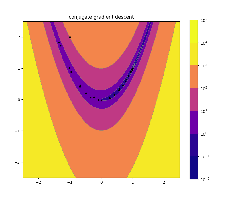
We mentioned earlier that the line search variant of gradient descent forces you to make 90 degree turns, leading to inefficient paths. Conjugate gradient descent relaxes the requirement that we move in the direction of steepest slope at each step, so that it can select directions that work well together.

Mathematically, it picks directions that are “conjugate”, meaning that for any two directions \(u_i\) and \(u_j\), \(u_i^T H u_j = 0\) where \(H\) is the Hessian matrix. Practically speaking, this ends up meaning that when we do a line search along some direction, no future direction “undoes” any of our work. That is, we don’t have to do a second line search along any one direction, since the line searches along later directions are guaranteed to leave us at the minimum along previous directions. This works exactly for quadratic functions. In particular, if your objective is an \(n\) dimensional quadratic function, CGD will find the optimum in exactly \(n\) steps. For non-quadratic functions, it still usually ends up being a huge improvement over standard gradient descent (since a quadratic approximation is more accurate than a linear one). You just keep restarting the algorithm after it runs through \(n\) different conjugate directions. Check out how many fewer points there are in the picture below, compared to regular gradient descent.

The final thing to mention about CGD is that even though it is an optimal method for quadratic functions, and the definition of conjugacy involves the Hessian matrix, you never need to calculate second derivatives explicitly. This information is built up from successive evaluations of the gradient alone. (If you did know the Hessian matrix up front, you could jump to the bottom of a quadratic function in one step.) If you want to read more about CGD, I have a full derivation in my notes from The Nature of Mathematical Modeling last year.

L-BFGS

The Broyden-Fletcher-Goldfarb-Shanno algorithm is similar to CGD in that it exploits curvature information (i.e. the Hessian matrix) to choose smarter descent directions. Like CGD, it approximates the Hessian matrix rather than needing to be able to compute it explicitly. Unlike CGD, it stores the full estimated Hessian matrix (CGD only needs to store one additional vector besides the current direction and the current gradient). For high dimensional problems, this quickly becomes impractical since you need to store \(n^2\) numbers. Limited Memory Broyden-Fletcher-Goldfarb-Shanno is a variant of BFGS that addresses this by storing a limited resolution version of the Hessian matrix instead.