B-Splines and Mixes
A while ago I had a long conversation with Sam Calisch in the muddy about splines, and whether / not they would serve as a viable underlying representation for distributed motion controllers (or any motion controllers). The proposition was that modern microcontrollers are probably beefy enough (esp. with FPUs) to evaluate splines in realtime.
This would mean that we could bring all of the wonderful spline properties to our motion controllers: compression of complex curves via spline fit (which are normally linear segments), smoothly interpolated corners (where most motion controllers hit some instantaneous acceleration at a junction), and more rigorous ideas about acceleration control. Given that splines have analytic derivatives, we should be able to use those to calculate i.e. cornering accelerations.
All together splines seem to offer a more “mathematic” path / trajectory definition than line segments and trapezoids. Which was admittedly more Sam’s desire than mine, but I see it now.
Spline Primer
There are better spline nerds out there than I, and the wiki page is OK.
The topic can be vague and confusing because there are so many different types of splines, and many names. I’m barely even confident enough to make any claims, but AFAIK splines are basically just polynomial functions that describe curvatures. There are a handful of ways to arrive at different curves (relating “control points” to arrive at polynomial coefficients), and we typically see splines “chained together” to define paths. That is, these are piecewise polynomial functions.
General Cubic Spline
For example, we can have the extremely general cubic spline, which is literally just a cubic polynomial with coeffcicients $a_0, a_1, a_2, a_3$
$s(t) = a_0 + a_1t + a_2t^2 + a_3t^3, t \in [0, T]$
Since we have four parameters, we have four degrees of freedom. We can constrain these by setting i.e. the positions at the endpoints, and the 1st derivatives (slopes) at the endpoints:
$s(0) = 0 \;\;\; \dot{s}(0) = 0$
$s(T) = 1 \;\;\; \dot{s}(T) = 0$
Then we could find parameters that fit. However, we normally define these things (at least when we are using them geometrically) with control points. There’s a lot of different styles, I’m just going to look at two:
Cubic Hermite Spline
The “cubic hermite” spline is formulated in terms of endpoint positions $p_0, p_1$ and slopes $m_0, m_1$ -
$p(t) = (2t^3 - 3t^2 + 1)p_0 + (t^3 - 2t^2 + t)m_0 +(-2t^3 + 3t^2)p_1 + (t^3 - t^2)m_1$
If we are defining some motion path and know our current position and velocity, but want to interpolate to a new one, this is obviously useful.
Catmull-Rom Spline
These are famous in computer graphics - Catmull is one of the founders of Pixar. There’s a good wikipedia article on the topic. Catmull-Rom splines are a form of cubic hermite.
And, oddly, there seems to be a better approach in this youtube video. Here we describe some list of points $p_0, p_1, p_2, p_3$ and basis functions that form ‘field of influence’ over the curve segment. Here are the basis functions:
$y_1 = -x^3 + 2x^2 - x$
$y_2 = 3x^3 - 5x^2 + 2$
$y_3 =-3x^3 + 4x^2 + x$
$y_4 = x^3 - x^2$
And to generate some point on the interval between $p_1, p_2$ we seem to have:
$x(t) = 0.5(p_0*y_1(t) + p_1 * y_2(t) + p_2 * y_3(t) + p_3 * y_4(t))$
Where we take each point by it’s “influential field” and have this whole thing to 1/2 as the basis functions above span 0-2.
def y0(x):
return -x**3 + 2*x**2 -x
def y1(x):
return 3*x**3 - 5*x**2 + 2
def y2(x):
return -3*x**3 + 4*x**2 + x
def y3(x):
return x**3 - x**2
def catmull(p0, p1, p2, p3, s):
return 0.5 * (p0 * y0(s) + p1 * y1(s) + p2 * y2(s) + p3 * y3(s))
# np array multiplcation is rad,
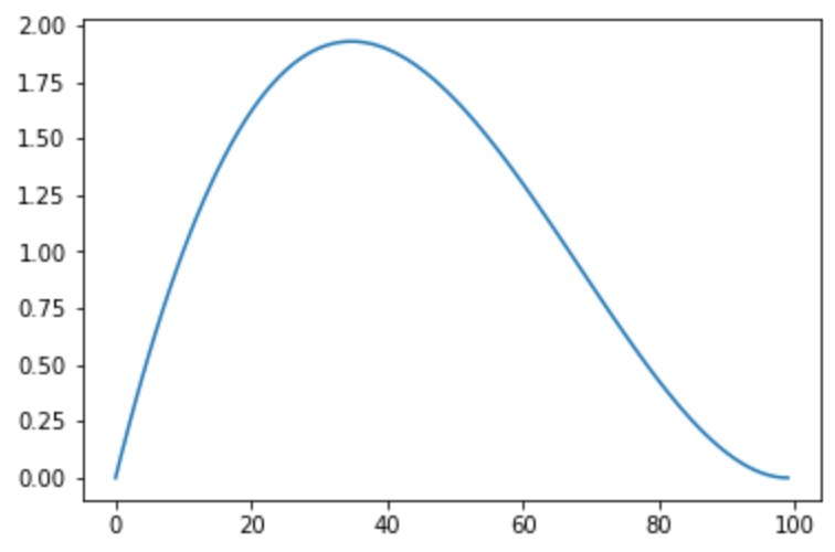
s = np.linspace(0, 1, 100)
pts = catmull(0, 2, 1, 0, s)
plt.plot(pts)
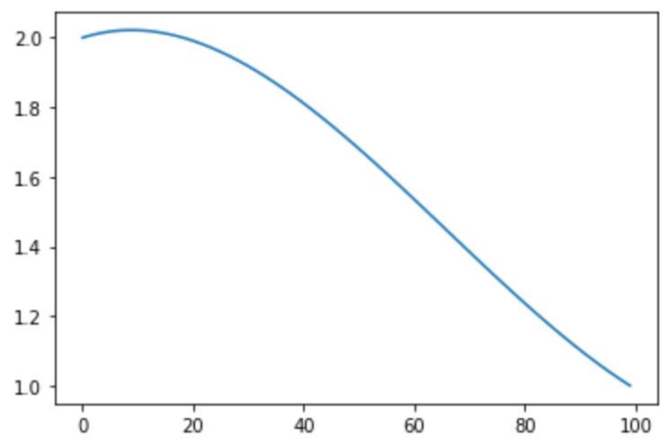
Cubic Bezier Curve
Beziers are similarely simple in formulation: though where a catmull-rom spline will go through each control point, a bezier only passes through endpoints. By the way the bezier wiki is awesome.
In the cubic case, we can think of the endpoints, well, as endpoints, and the other two points as setting slopes at those endpoints. This is a similarely handy formulation.
For a segment between $P_0, P_1, P_2, P_3$ not reaching $P_1, P_2$ - and for some $P_1, P_2$ the curve may be self intersecting. Careful with that one then.
Explicitly,
$B(t) = (1-t)^3P_0 + 3(1-t)^2tP_1 + 3(1-t)t^2P_2 + t^3P_3$
We also have the first derivative
$ \dot{B}(t) = 3(1-t)^2(P_1 - P_0) + 6(1-t)t(P_2-P_1) + 3t^2(P_3 - P_2) $
And the second derivative:
$ \ddot{B}(t) =6(1-t)(P_2 - 2P_1 + P_0) + 6t(P_3 - 2P_2 + P_1) $
Note that these plots are just in 1D, where the x axis is samples (so is really 0-1, on the curve’s “parameterization”).
def cubicBezier(p0, p1, p2, p3, s):
    return (1-s)**3*p0 + 3*(1-s)**2*s*p1 + 3*(1-s)**2*s**2*p2 + s**3*p3
cpts = cubicBezier(0, 4, 1, 0, s)
plt.plot(cpts)
Splines in Py
Given some basic spline understanding, I wanted to look at how I might use these to chain together motion controllers. To start, I wrote some spline classes. I am using Beziers because I suspect (as does Sam) that a cubic bezier is the best representation to eventually send to the motor (or perhaps just a generalized cubic) - they allow us to define positions & velocities at endpoints, this is about as much information as we should need.
# make a cubic bezier
class cubic:
    def __init__(self, p0, p1, p2, p3):
        self.p0 = p0
        self.p1 = p1
        self.p2 = p2
        self.p3 = p3
        self.len = self.getLen()

    # get point from og 0-1 parameterization
    def xs(self, s):
        return (
            (1 - s) ** 3 * self.p0
            + 3 * (1 - s) ** 2 * s * self.p1
            + 3 * (1 - s) * s ** 2 * self.p2
            + s ** 3 * self.p3
        )

    # first derivative
    def xdots(self, s):
        return (
            3 * (1 - s) ** 2 * (self.p1 - self.p0)
            + 6 * (1 - s) * s * (self.p2 - self.p1)
            + 3 * s ** 2 * (self.p3 - self.p2)
        )

    # second derivtaive
    def xddots(self, s):
        return 6 * (1 - s) * (self.p2 - 2 * self.p1 + self.p0) + 6 * s * (
            self.p3 - 2 * self.p2 + self.p1
        )

    # integrate over length
    def getLen(self, samples=10000):
        s = np.linspace(0, 1, samples)
        length = 0
        last = self.p0
        for i in range(len(s)):
            length += np.linalg.norm(last - self.xs(s[i]))
            last = self.xs(s[i])
        return length

    # get point from 0-length along
    def xl(self, l):
        if l > self.len:
            return False
        return self.xs(l / self.len)

    # get speed from 0-length
    def xdotl(self, l):
        if l > self.len:
            return False
        return self.xdots(l / self.len) / self.len

    # get accel from 0-length
    def xddotl(self, l):
        if l > self.len:
            return False
        return self.xddots(l / self.len) / self.len
However, there’s also going to be a lot of lines. Straight ones. So I have a class for these as well:
# make a linear bezier (... a line)
class linear:
    def __init__(self, p0, p1):
        self.p0 = p0
        self.p1 = p1
        self.len = self.getLen()

    # pt on lin
    def xs(self, s):
        return (1-s)*self.p0 + s*self.p1

    # get length, can do direct...
    def getLen(self, samples = 10000):
        return np.linalg.norm(self.p1 - self.p0)

    # get first derivative,
    def xdots(self, s):
        return self.p1 - self.p0 # not sure about this, should it be unit vector ?

    def xddots(self, s):
        return self.p0 * 0 # fairly sure about that, use self.p0 to return np zeroes of dof

    # pt from 0->length
    def xl(self, l):
        if(l > self.len):
            return False
        return self.xs(l / self.len)

    def xdotl(self, l):
        return self.xdots(l / self.len) / self.len # checks out for velocity = 1 case,

    def xddotl(self, l):
        return self.p0 * 0
Given these classes I can make paths that are chains of curve-defining classes. Here, I add four points around junctions (corners) to define a bezier curve around the corner. This means I have genuine smoothness around corners instead of “fake” junction deviation as used in GRBL. As a note: these will become very small in real implementations (!).
So, here, in green are the OG control points, red are added points to define cubic beziers at corners:
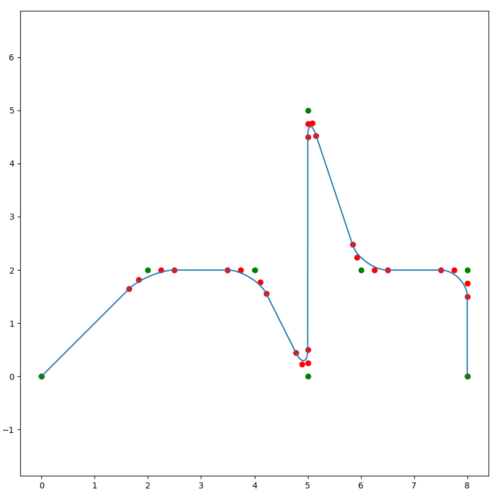
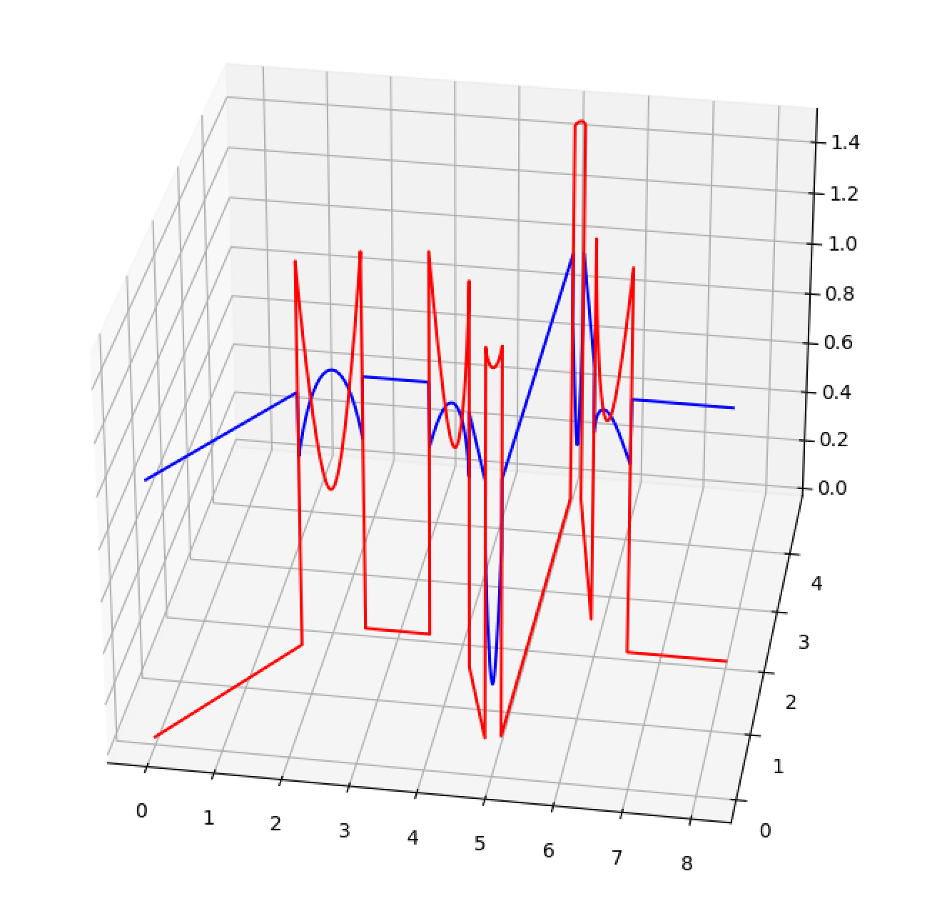
Now I can use the spline classes first and second derivatives to look at accelerations and velocities around the corners. I’m less sure about these, but they seem to make some sense. Below, the blue plots velocities in z, the red plots accelerations in z:
Between Bezier Parameterization and Real Space
There is a major trap here - beziers (and indeed most of these) are evaluated in $[0:1]$ but have real “lengths” in some space (in this case) through $x,y$ - or whatever DOF the system has. There’s no closed form solution for the integral of a cubic bezier, so the easy way is to do this with a brutal discrete integration:
def getLen(self, samples=10000):
    s = np.linspace(0, 1, samples)
    length = 0
    last = self.p0
    for i in range(len(s)):
        length += np.linalg.norm(last - self.xs(s[i]))
        last = self.xs(s[i])
    return length
And then this length can be used to scale position lookups along the curve’s real length:
def xl(self, l):
    if(l > self.len):
        return False
    return self.xs(l / self.len)
This is part of the larger problem here: we have nice curves in $[0:1]$ but our dynamics (which we want to link to our path definition) occur in the geometric space the curve defines. I’m obviously still grappling with this.
The thing I was surprised by is that velocity through the bezier is not constant in xy. It is worth noting that they are parabolic, which is also obvious if we look at the quadratic form of their first derivative. This is seen in the 3D plots above, and is the first struggle for the next section:
Time Scaling & Dynamics
It’s worth looking for a minute at why we’re interested in this. The notion here is that we can use our mathematic path definition with a mathematic definition of our system dynamics (!) to generate an optimal path trajectory.
So, to back up a minute, each of our position DOFs has some actuator with a torque curve that we could say is related to it’s angular velocity. In thisnorthwestern video on path generation they are formulated in terms of angular velocities and positions, so for each motor $\tau_i$ we have the constraint that at any point:
$\tau_i^{min}(\theta, \dot{\theta}) \leq \tau_i \leq \tau_i^{max}(\theta, \dot{\theta})$
That is, we don’t exceed the motor’s minimum (negative) or maxmum (positive) torque, which is itself a function of that actuator’s current angular position and (more importantly) speed. In any case, suffice it to say that “we have some model of the machine’s dynamics”
What we want to do, then, is walk our path and determine where we need to slow down and also where we can speed up to minimize traversal time through the path while respecting actuator constraints - this is the grail we are after here.
With these things linked, we are also more likely to build a model wherein we could learn system dynamics based on the resulting torques required to navigate one of these paths.
From the video noted, there’s some great insight on how this is normally done.
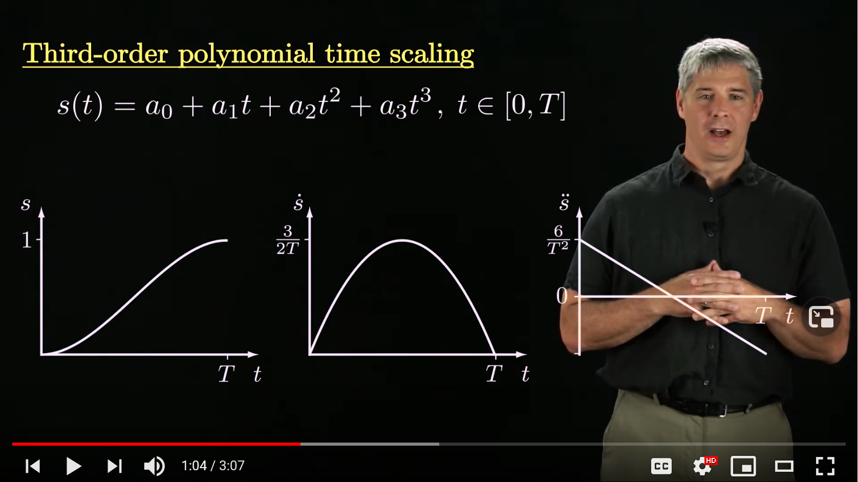
First, we apply some time scaling to each segment, this is another but different cubic spline in time space:
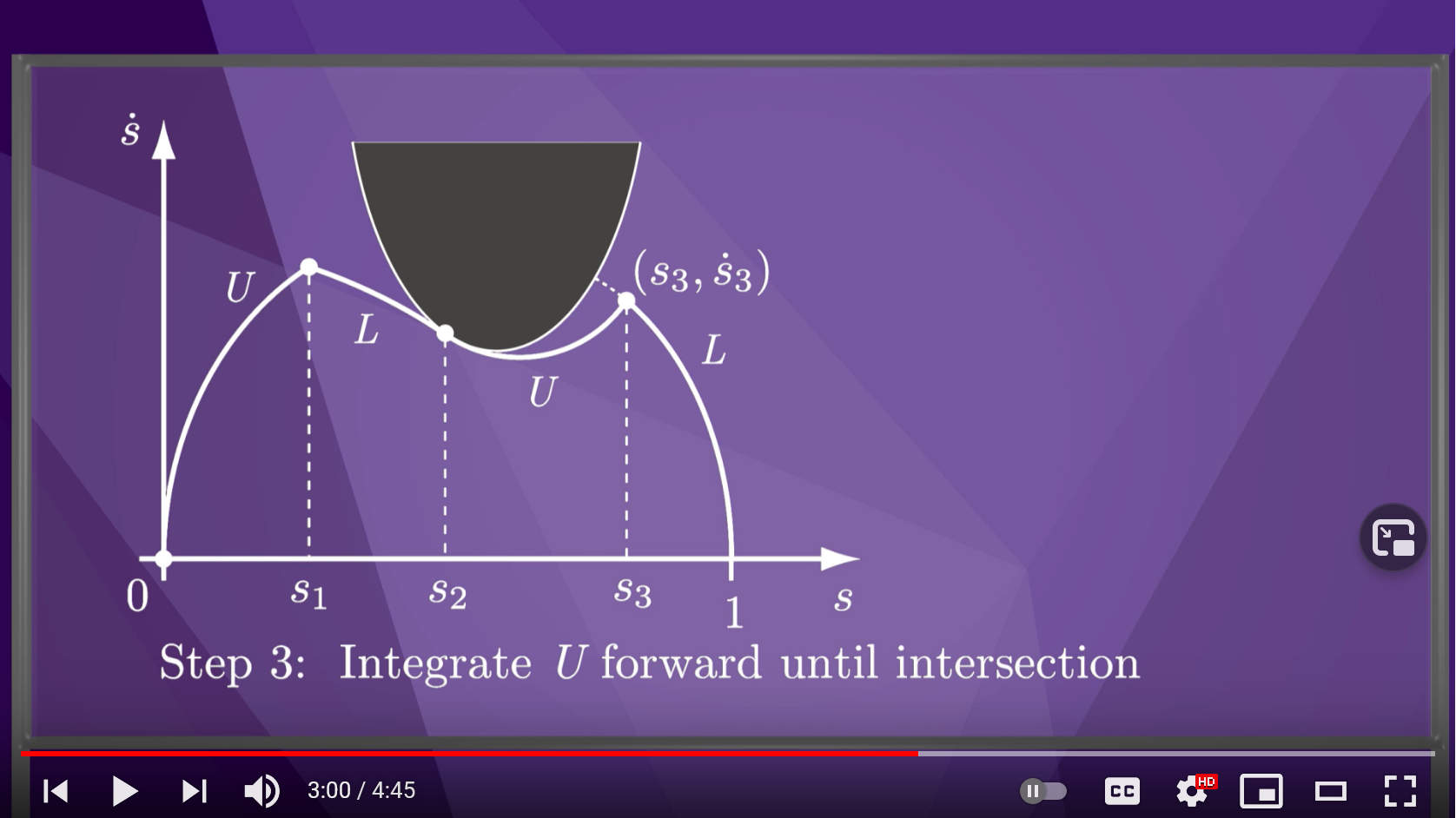
Now we want to find this time scaling, and (I’m at a loss as to how) but we find these by forward integrating along the path, under constraints of our dynamics, on the edge of maximal acceleration. That means at each step in the path (assuming some start condition) we walk forwards, picking the maximal motor torque available, that will send us along the curve. This will have us hit the end of the path at some large velocity, but we probably want to be coming to a stop under our deceleration constraints, so we also reverse integrate choosing minimal (stopping) accelerations.
Then, we can find the point these intersect:
And apply the resulting time scaling to our path, to have a “trajectory” - path w/ speeds.
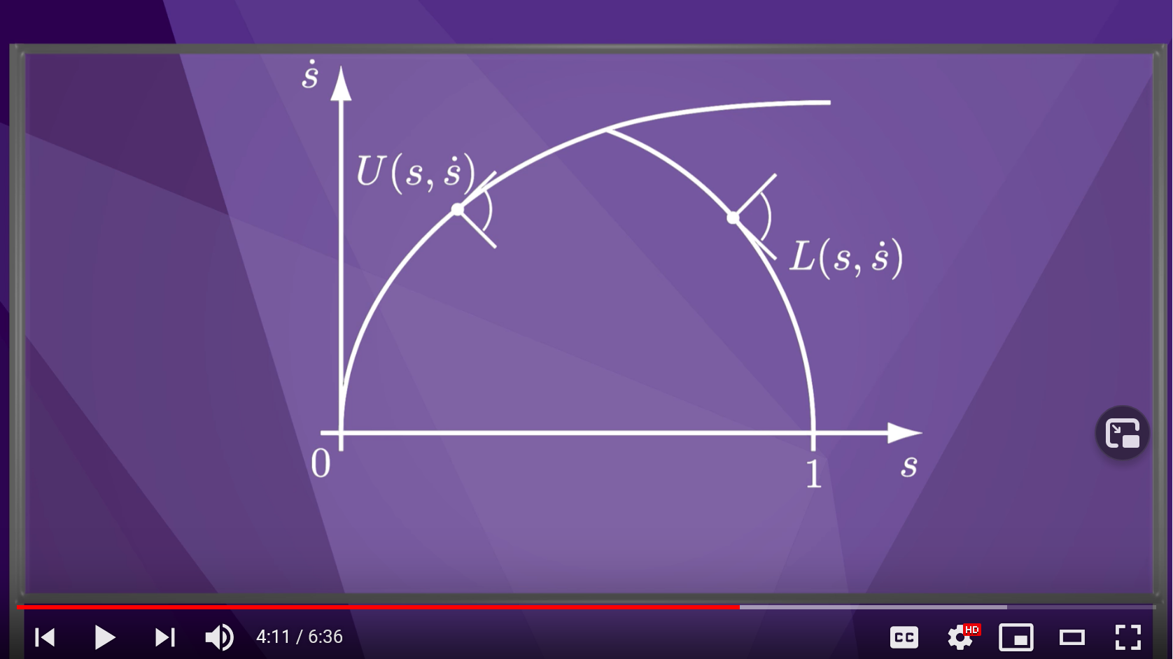
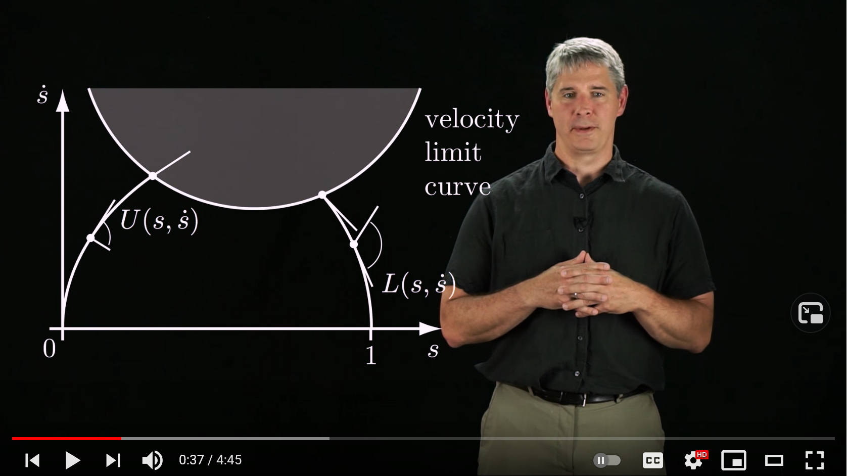
However, there’s an extra trap in here: we can’t accelerate forever, we’ll have some “velocity limit curve” and we can’t just do a dead-run into this as well, or we’ll exceed the limit:
So we also need to do some search to find an optimal path that touches tangentially this curve:
So, the dynamics work is what I’ll be getting into next. I am curious if perhaps a simple discrete method will end up serving better than full on analytic linkages: as I suspect I will want to stack models on models, and it will perhaps be easier to simply step through these things in discrete time than to try to hook all of the derivatives up, etc.
Possible Architectures
So, what about actually getting to the motors? This is where I started. We supposed that the cubic spline was a great motor-level “move” representation because it allows us to “compress” some long-ish interval of time into one data packet, and it allows us to set positions and velocities at the ends of those points: and the curve generates accelerations in between them. Whether this is a spline in velocity & time or in position & time is something I have yet to understand, nor how we generate these splines given system dynamics.
However, an architecture might look like:
| step | where | notes |
|---|---|---|
| input path | anywhere | line segments, arcs (which are well approximated with cubic beziers), n-dof vectors |
| spline fitting | python / numpy | fit junctions, etc, to path: build underlying rep. of path as spline chain |
| time scaling against dynamic limits | python / numpy | use machine dynamics model, cartesian : actuator transforms, etc, to fit a time scale to path to generate a dynamics-respecting trajectory |
| actuator spline generation | python / numpy | write vel/time, or pos/time splines that motors can interpret |
| spline execution | motor / actuator | motors buffer cubic splines in whatever space, time-integrate them at high frequency to generate and go-to positions |
| spline response | motor / actuator | motor simultaneously generates reciprocal spline fit to torques / effort required to follow spline: use this to feedback / fit dynamics model which is doing the planning |