Computational Geometry

Both disciplines of path planning are based on processing geometric information, so to get started it’s helpful to look at the various ways we might do this.

Representations

1D - Curves

Ultimately the path that a tool or robot takes is some one dimensional curve parametrized by time. Usually the path is embedded in three dimensional space, though for some toolpathing operations we’ll only need two. Often to start we’ll just care about the geometry of the curve, rather than the speed(s) at which it is traversed. To represent a curve’s geometry, there are many common options.

Points/Line segments: Just explode the path into a bunch of points, implicitly connected by line segments. Despite the simplicity, with enough points you can approximate any curve to arbitrary accuracy.

Line segments and Other Primitives: We can add add some other primitives to our line segments. Arcs are the most common addition.

Splines: There are a lot of different splines, which ultimately are all ways to parametrize curves with different forms of polynomials (or ratios of polynomials). Splines are named after the wooden tools that were used by architects and boat builders (among others) to repeatably draws curves before all these newfangled computers.

• B-Spline
• Bezier Spline
• Cubic Hermite Spline (and Catmull-Rom Spline)
• Jake’s Spline Primer

Implicit Curves The level sets of an algebraic expression of x and y are one dimensional curves. Algebraic expressions of x, y, and z can determine curves if we add an additional constraint (e.g. the expression has some fixed value, and z has some other fixed value).

Discretized Points Finally, we can use simple line segments, but constrain the points to lie on the vertices of some lattice. As we will see, doing so can drastically change the nature of the relevant path planning algoritms, since we will be solving discrete problems instead of using floating point numbers to approximate real numbers (sometimes quite poorly despite our best efforts). Note that if your machine uses steppe motors (and you drive them in individual steps), then physically the configurations of your machine’s axes are discretized (unless we want to start modeling backlash, deformation, etc.).

2D - Surfaces

When designing parts, it’s often helpful to define features on specific surfaces rather than letting them float around in three space arbitrarily. The same is true for toolpathing operations.

Meshes The analog of connecting points with line segments to form 1D curves is to connect points with sections of planes to form 2D surfaces. Often meshes are restricted to use triangles, but you may also see quad, hex, or mixed meshes.

Point Clouds If we take a mesh and throw away the connectivity information (which points should be connected to form triangles), we’re just left with the points. Sometimes this is all we need. Other times, it’s all we get, as with many 3D scanning techniques. We’ll see algorithms for stitching point clouds into meshes later.

Higher-Order Meshes If the discontinuities in surface normals between the triangles (or quads, etc.) in your mesh become problematic, and you don’t want to add a ton more triangles, you can use higher order surfaces instead of linear ones to generate meshes with real curvature.

Fixed Point Meshes We can constrain the points used to define our mesh to lie on the vertices of a lattice (and use fixed point numbers instead of floating point numbers to represent coordinates).

Other Primitives Just as we combined arcs with line segments in 2D, we can add sections of surfaces like cylinders and cones to the planar sections commonly seen in meshes. The boundaries between primitives necessarily end up being more complex than in meshes (i.e. not just line segments), since cylinders and cones aren’t planar.

Splines Splines work just as well for 2D objects as they do for curves. All of the splines we’ve seen so far can be generalized to 2D.

• NURBS (NURBS can be used to represent 2D, 3D or any other dimensional shape, but are most commonly used for 2D surfaces.)

Implicit Surfaces The level sets of an algebraic expression involving x, y, and z (or some other three dimensional coordinate system) are 2D surfaces.

3D - Volumes

Meshes We can keep generalizing the “connect points with linear elements” strategy. To represent a volume, we just use meshes of 3D objects like tetrahedra instead of 2D objects like triangles (or 1D objects like line segments).

Fixed Point Meshes We can constrain the points used to define our mesh to lie on the vertices of a lattice (and use fixed point numbers instead of floating point numbers to represent coordinates).

Point Clouds Again, we can also just sample a bunch of points from within a volume. Among other things, this is useful for seeding particle based simulations.

Boundary Representations (B-reps) When we’re working in three dimensions, any closed surface defines a volume. (Technically speaking we may also want to require that the surface is orientable, has no non-manifold geometry, and/or that it doesn’t intersect itself.) So we can use any of the above 2D representations to represent 3D shapes as well. Most common CAD programs use B-reps based on geometric primitives like planes and cylinders, augmented with splines and meshes.

Splines There’s no reason we can’t use splines with three parameters to directly describe volumes, but this isn’t used often in practice.

Implicit Volumes (F-reps) We can represent volumes directly with algebraic expressions of x, y, and z (or other three dimensional coordinate systems): instead of taking level sets, we consider regions where the expression is above (or below) some threshold (usually zero). A particular case is signed distance fields, in which the value at each point represents the distance from that point to the boundary of the volume, with negative values given for internal points.

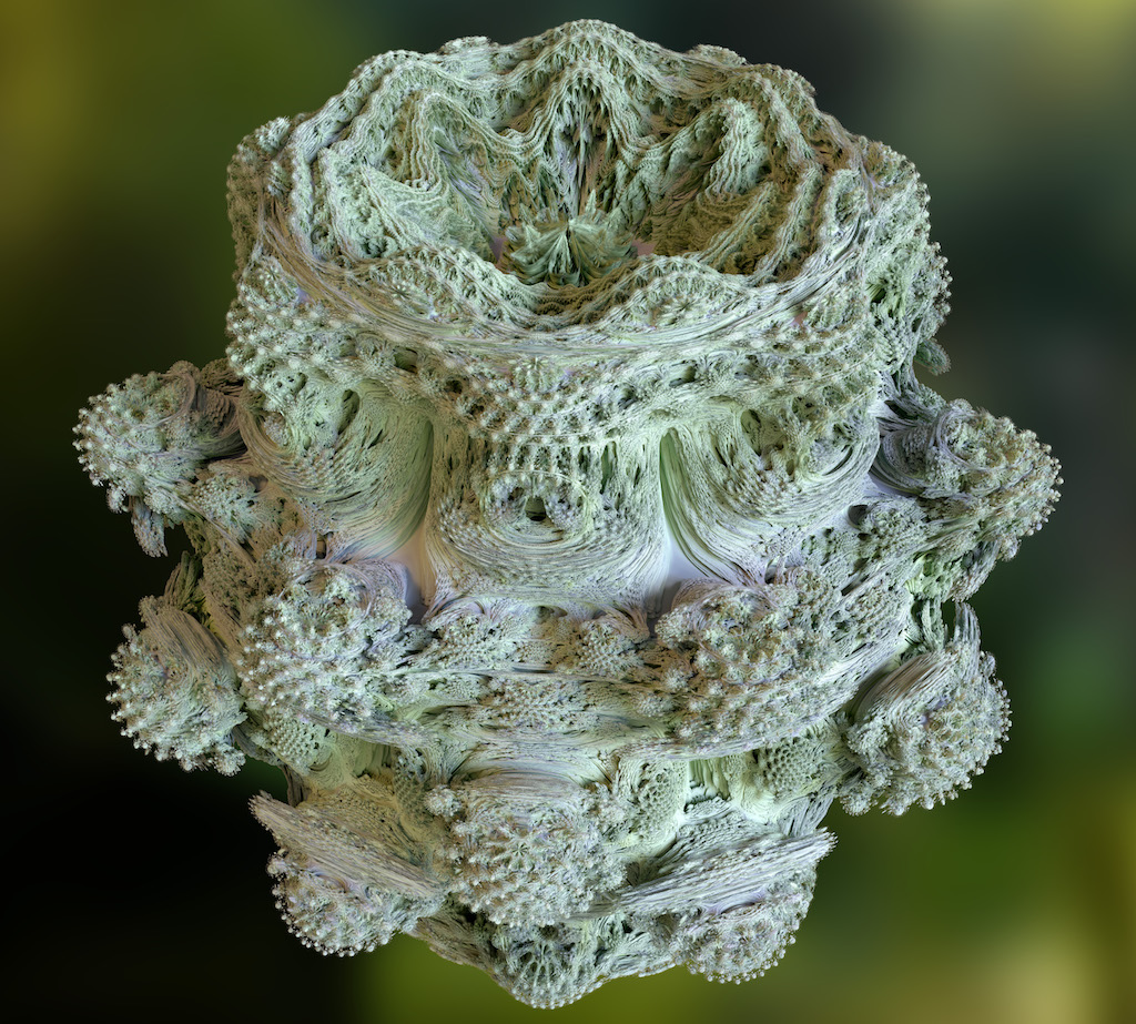
As an aside, there are other ways to represent volumes implicitly. Instead of thresholding a function from three space to the real line, we can take a function from three space to itself and consider the orbits of each point (i.e. what happens when we take a point, feed it through our function, then feed that point through the function, etc.). Probably the most well known shape defined in this manner is the Mandelbulb. I’ve never seen this sort of representation used for computational geometry.

Voxels If we discretize our space, usually into tiny cubes, then we can just specify which elements are in the shape and which are not. This is arguably the simplest representation format to describe and process, but it can end up being extremely memory intensive. As a result, various schemes exist to compress voxel data, usually using hierarchical data structures like octrees.

Adaptively Sampled Distance Fields This is a combination of signed distance fields and voxels (or pixels, if we do the same thing in 2D). The basic idea is to sample a signed distance field in the center of each voxel. To make it adaptive, we use an octree or some other hierarchical structure to compress the data, allowing the resolution to change as needed across the volume.

Algorithms

Points

• Distance between two points.
• Distance from a point to a line.
• Distance from a point to a plane. This is usually computed as a signed distance, which tells you on which side of the plane the point lies. (Of course for this to make sense you have to give the plane an orientation, as naturally occurs if you represent a plane with its normal vector.)
• Checking whether a point is contained by a box, cylinder, etc.
• Finding the convex hull of a collection of points.

All of these algorithms except the last are constant time; finding a convex hull has n log n complexity in the number of points.

Lines

• Checking intersections of a set of line segments (in 2D).
• Points of closest approach between two lines (in 3D).
• Ray/triangle intersections: does a ray intersect a triangle, and if so, where.
• Intersections of rays with other primitives (boxes, cylinders, cones, etc.)

Triangles

• Finding intersections of triangles (i.e. the line segment or possibly plane they share, if any).
• Delaunay triangulation of a set of points. This gives the “best” triangulation, where best is defined as maximizing the smallest angle among all the triangles. This gives you triangles as close to equilateral as possible, as opposed to long skinny triangles. You can also use the Delaunay triangulation to construct the Voronoi diagram, i.e. the boundaries of the territories closest to each point.

• Triangulating a polygon. We can think of this as converting a representation of a (closed) curve into a surface mesh. Often we want the resulting mesh to be “high quality”, usually meaning that it is Delaunay, nearly Delaunay, or – stricter yet – has a given minimum angle size (which is only possible when you get to add new points). Jonathan Shewchuck’s Triangle library is a great resource for all things triangulation related.

Discretization

• Bresenham’s Algorithm. It may seem trivial, but a foundational algorithm for computer graphics that also comes up in computational geometry is for making the best rasterized approximation of a line.

• Midpoint Circle Algorithm. This is the equivalent of Bresenham’s Algorithm for circles.

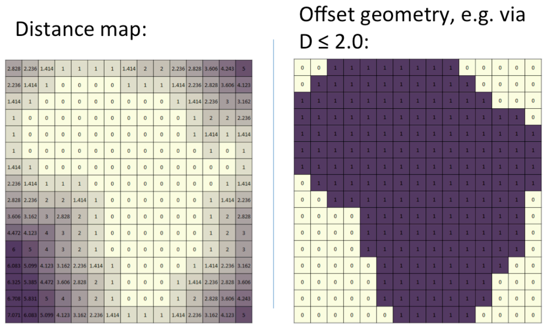
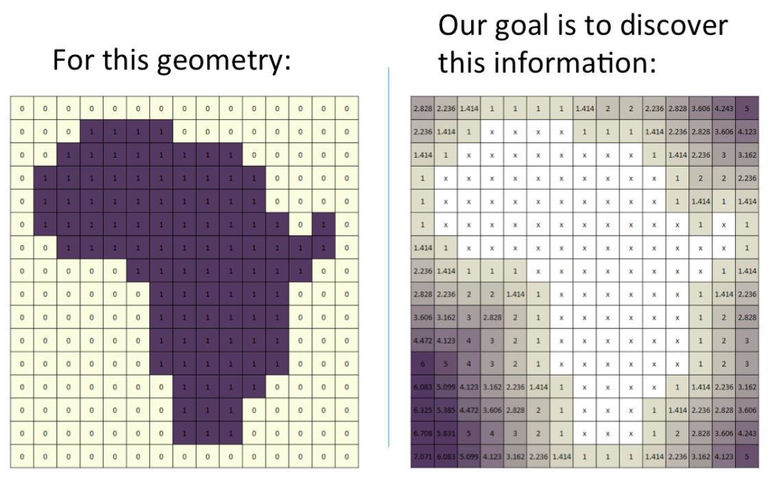
• Distance Transform. This algorithm turns a binary inside/outside representation for pixels (or voxels, in 3D) into a uniformly sampled distance field. See Meijster et al. 2002. An easier introduction (and the source of the image below) is provided in the path planning notes from 2012.

Offsets

A useful thing is to be able to create a new curve that is offset by a constant distance from another. The way you do this depends on what geometry representation you’re using.

Line segments and circles are easy to offset individually, so the only challenge in making offset curves of line and arc curves is in checking when portions of offsets “get too small” and disappear. Splines have similar algorithms, though they generally only generate approximate offset curves (accurate to a specified tolerance), and are more complicated.

If you have a distance field, you’re in luck. Instead of finding the level surface with value 0, just find the level surface of the desired offset. This works for analytic and discretized distance fields.