Robotic Path Planning

Robotic path planning is trying to answer a different question from the previously discussed toolpath planning - instead of removing or adding material to fabricate an object, robotic path planning determines how an object can navigate through a space with known or unknown obstacles while minimizing collisions.

Map representation

Robots are either given, or implicitly build, a mapped representation of their surrounding space. This map can be saved as a discrete approximations with chunks of equal size (like a grid map) or differing sizes (like a topological map, for example road-maps). Continuous map approximations can also be stored by defining inner and outer boundaries as polygons and paths around boundaries as a sequence of real valued points. Although continuous maps have clear memory advantages, discrete maps are most common in robotic path planning because they map well to graph representations which have a rich history of search and optimization algorithms with simple computation complexity.

Occupancy grid maps discretize a space into square of arbitrary resolution and assigns each square either a binary or probabilistic value of being full or empty. Grid maps can be optimized for memory by storing it as a k-d tree so that only areas with important boundary information need to be saved at full resolution.

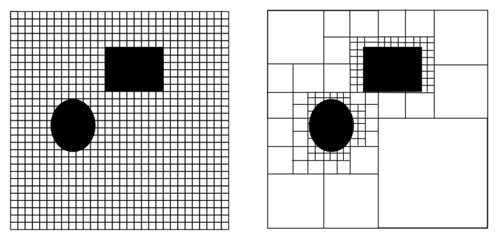
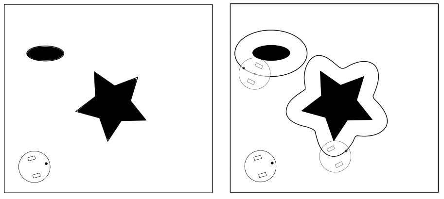
Configuration space: To deal with the fact that robots have some physical embodiment which requires space with in the spatial map, configuration space is defined such that the robot is reduced to a point-mass and all obstacles are enlarged by half of the longest extension of the robot.

Tree search algorithms

Once a space is represented as a graph, there are classic shortest-path graph algorithms that can guarantee the shortest path is found, if given unlimited computation time and resources.

Dijkstra’s algorithm (1959)

Dijsktra’s algorithm creates a set of “visited” and “unvisited” nodes. An initial starting node is assigned a distance of zero and all other node’s distance values are set to infinity. Then, each neighbor is visited and it’s distance from the current node is determined, if the distance is less than the previously defined distance value, then the value is updated. Once all neighboring values are updated, the algorithm moves the current node of the “visited” set and repeats the process of the next neighboring node with the shortest distance value. The algorithm continues until all nodes have been moved from “unvisited” to “visited”.

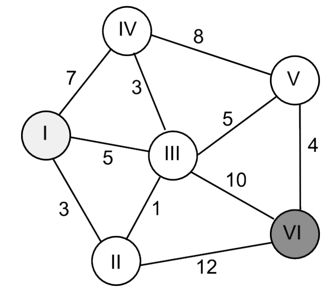
For example, Dijkstra’s algorithm used to find the shortest path from I to VI in the above graph would behave as follows:

• from node I: IV=7, III=5, II=3
• from node II: III=3 + 1=4, VI=3 + 12=15
• from node III: IV=4 + 3=7, V=4 + 5=9, VI=4 + 10 = 14
• from node IV: V= 7 + 8 = 15
• from node V: VI = 9 + 4 =13, update VI to 13 because it’s shortest

Therefore, I->II->III->V->VI is determined to be shortest.

A* (1968)

A* is another path-finding algorithm that extends Dijkstra’s algorithm by adding heuristics to stop certain unnecessary nodes from being searched. This is done by weighting the cost values of each node distance by their euclidean distance from the desired endpoint. Therefore, only paths that are headed generally in the correct direction will be evaluated.

D* (1994)

D* is an incremental search algorithm, meaning that it uses information from previous algorithm searches to speed up exploration of the space. When combined with A*, D* allows for faster re-planning around objects by adding more heuristics to account for obstacles. Instead of a specific algorithm, D* more generally refers to search algorithms that combine incremental speed ups with A* heuristic approaches.

Sampling-based planning

In reality, most algorithms do not need to reach full completion to find a reasonable path and doing so would be too computationally expensive. Therefore, most algorithms are resolution complete meaning that the algorithm is only as complete as the state-space is and discretization can play a large role in the accuracy of the result.

Sampling based planner are probabilistic complete, meaning that they create possible paths by randomly adding points to a tree until the best solution is found or time expires - as time approaches infinity, the probability of finding the optimal path approaches 1.

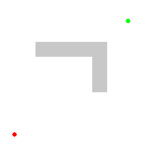
Rapidly-exploring random trees (RRT) (1998)

RRT quickly searches a space by randomly expanding a a space-filling tree until the desired target point is found. The basic algorithm is as follows, for some starting point, start, and a ending goal, goal

tree = init(x, start)
while elapsed_time < t and no_goal(goal):
    new_point = stateToExpandFrom(tree)
    new_segment = createPathToTree(new_point)
    if chooseToAdd(new_Segment):
        tree = insert(tree, new_segment)
return tree

• stateToExpandFrom(): finds the next into to add, which can be completely random search over the state space or can be informed by preferences around nodes with fewer out-degrees (i.e. less connections)
• createpathToTree(): this can use the classical shortest-distance graph algorithm for mapping a points to the tree, but that does necessarily choose the overall shortest path. RRT* is an extension of RRT which connects the point in a way that minimizes the overall path length - this is easiest to do when starting from the goal instead of the starting point.
• chooseToAdd(): needs to check for collisions which can be the most computationally expensive part, especially if the robot can run into itself. There are tricks for “lazy collision evaluation”, which only checks for collisions at suitable paths, and if a collision occurs then just that bad segment is deleted, while the rest of the path remains.

intense RRT in 12-dimensional state-space from Steve LaValle and James Kuffner in 2000, here:

Machine Learning path planning

Machine learning methods are the latest development for determining robotic path planning. Reinforcement learning using Markov Decision Processes or deep neural networks can allow robots to modify their policy as it receives feedback on its environment. Classical Q-learning algorithms provide a model free learning environment.

These methods were explained in beautiful detail on the previous week’s control theory page.

• Deep learning motion planning for smooth control of grasping (Inchnowski et.al. 2020)

• Robots following a line on the floor with smooth PID control - more control theory, but closely related to real-time path planning

• Robots also fail all the time

• and for compeltion, Boston Dynamics 2020 dancing robots