


Final_files/shapeimage_5_link_0.png)
Final_files/shapeimage_5_link_1.png)


Here’s what happened ...
What it does
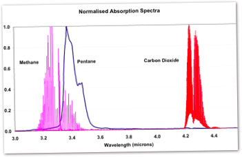
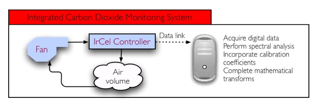
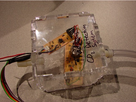
The system detects carbon dioxide concentrations within an open or closed airflow loop and displays those readings in real-time on a PC. The system operates by means of infrared spectrum analysis.
System diagram
The system diagram is as follows:
Fabrication processes
* Lasercutter was used to create an enclosure which can be made airtight
* Low-temperature wax was used as a sealant to secure air and data ports on the side of enclosure
* PCB design was used extensively to create the necessary circuitry
* Software development (assembly and Python) was required to process the raw infrared spectrum data and generate a representation of the carbon dioxide concentration
Listing of materials and components
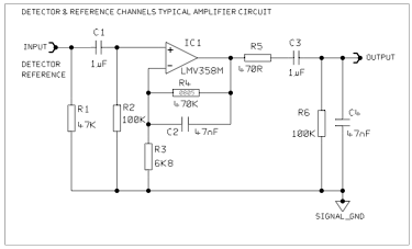
The IrCel circuit diagram is as follows (manufacturer-supplied). It uses a high-precision rail-to-rail op-amp (LMV358M) together with several RC bridges to
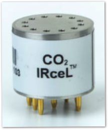
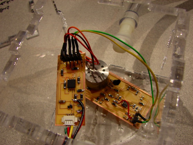
The City Tech IrCel sensor was installed according to the above circuit diagram, mounted on a custom-made PCB. Sensor data is acquired by the microcontroller ADC on 2 channels at 1kHz. The ADC transmit raw data values the PC which subsequently performs spectral analysis and calculations to generate an actual atmospheric CO2 reading.
NOT SO SIMPLE ...
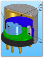
The sensor has to be driven by an externally-supplied square wave which pulses the internal IR lamp. The sensor generates two analogue output voltages (“detector” and “reference”), each of which oscillates at the lamp drive frequency which must be externally supplied. The manufacturer recommends a 5V square wave oscillating at 2Hz for best performance. Typically with a 5V DC supply an output of <30mV peak to peak will be seen. This waveform is amplified and passively filtered by the circuitry shown above.
The process of obtaining actual carbon dioxide concentration is lengthy and involved. First, the amplified “det” and “ref” signals are sampled at a rate of 1kHz. The absolute magnitude of each of these signals must then be integrated over a complete lamp cycle, before the following mathematical operations are performed:
Fractional Absorbance
A ratio of the gas to reference channels is required to give an accurate gas concentration over time. For this reason the actual units of the raw data are of no importance. The ratio at the last zero setting point is stored by the manufacturer in the on-board EEPROM where it is listed as variable “ZCC.” It is used as a baseline reference data point.
To calculate the fractional absorbance the following formula is used:
FA = 1 - (gas / (ref * ZCC))
where:
FA Fractional Absorbance
gas Gas channel data, amplified and magnitude averaged over a single period
ref Reference channel data, amplified and magnitude averaged over a single period
ZCC Gas Zero Constant (from EEPROM data)
Zero Temperature Correction
To account for variations in the performance of the detector/ lamp arrangement with temperature with respect to the zero point, the zero temperature and zero correction coefficients can be used. To calculate the zero temperature corrected fractional absorbance, the following formula is given:
ZTFA = FA - ZTC * (temp - ZTP)
where:
ZTFA Zero Temperature corrected Fractional Absorbance
FA Fractional Absorbance
ZTC Zero temperature coefficient (from EEPROM)
temp Temperature of sensor in °C, using internal thermistor
ZTP Temperature during zero operation (from EEPROM)
Span Temperature Correction
To account for variations in the performance of the detector/ lamp arrangement with temperature with respect to the span point, the span temperature and span correction coefficients can be used. To calculate the span temperature corrected fractional absorbance, the following formula is given by the manufacturer:
STFA = ZTFA - STC * (temp - STP) * ZTFA / (SFA + ZTC * (temp - ZTP))
where:
STFA Span Temperature corrected Fractional Absorbance
ZTFA Zero Temperature corrected Fractional Absorbance
STC Span temperature coefficient (from EEPROM)
temp Temperature of sensor in °C, using internal thermistor
STP Temperature during span operation (from EEPROM)
SFA Span fractional absorbance (from EEPROM)
ZTC Zero temperature coefficient (from EEPROM)
ZTP Temperature during zero operation (from EEPROM)
Span Scaling Factor
Following temperature correction the fractional absorbance should be scaled using the span gas constant as follows:
FA = STFA * SCC
where:
FA Fractional Absorbance
STFA Span Temperature corrected Fractional Absorbance
SCC Gas Span Constant (from EEPROM)
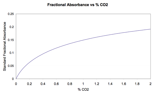
Standard Growth Curve
Finally the gas concentration can be calculated using standard growth curves as follows:
Gas = ( A.FA.FA + B.FA) / (C - FA)
where:
Gas Gas concentration (carbon dioxide in percent)
FA Fractional Absorbance (from Span Scaling Factor)
A Standard growth coefficient A, given by manufacturer as 3.10933
B Standard growth coefficient B, given by manufacturer as 0.5602
C Standard growth coefficient C, given by manufacturer as 0.30204
Reading the EEPROM
The EEPROM operates on Dallas Semiconductor’s 1-wire protocol. I read it using a PC interfacing adapter which I found in my lab. The results were as follows:
00 C8 analog span: 200
00 32 low alarm: 51
00 96 high alarm: 150
3F 90 F4 C7: ZCC, 1.13247
3F 6A 68 27: SCC, 0.91565174
B9 51 CD B3: ZTC, -2.0008422E-4
00 E7: ZTP, 231
39 AF 73 38: STC, 3.3464446E-4
00 E7: STP, 231
3E 3E 07 23: SFA, 0.1855741
Assembly Code Challenges
The requirements for the microcontroller were as follows:
-
1.Provide regulated 5V power to the IrCel
-
2.Generate a 5V 2Hz DC square wave to activate the IrCel’s infrared lamp unit
-
3.Acquire data on two channels, waveforms expected to be about 1V peak-to-peak
-
4.Data must be acquired with the greatest accuracy possible (given 10-bit ADC)
-
5.Data must be acquired at a rate of not less than 1000Hz
-
6.Individual data samples must be acquired at regular intervals, i.e. each sample separated by approximately 1 millisecond
-
7.Data must be transmitted with appropriate framing in real-time over a serial connection
To meet the above requirements, it was necessary to move to the Tiny45 microcontroller and initiate high-speed serial communications at 115200bps. The data rate constraints required nop-hacking to get the timing correct.
Data acquisition proved a major challenge. Initially I thought I could use the ADC’s bipolar differential mode to acquire the amplified waveforms from the IrCel. Unfortunately, given the fact that the ADC is only physically capable of acquiring voltages between 0V and 5V and given that the system provides the ground lead to the IrCel in the first place, this proved an incorrect strategy. Eventually I settled on rebiasing the waveforms about +0.5V and using the 1.1V ADC internal reference on the Tiny45 to successfully acquire data.
Python Challenges
The requirements for the PC front-end were as follows:
-
1.Provide graphical interface to user
-
2.Provide evidence that system is operational (waveform visualisation)
-
3.Capability to write data to file for subsequent offline analysis
-
4.Perform calculations as described above, according to manufacturer’s specifications, to take waveforms and convert them into a final result.
-
5.Real-time numeric output of atmospheric carbon dioxide concentration
The primary challenge in meeting the above requirements was incorporating Python Numeric and Math libraries to perform the necessary calculations using the coefficients extracted from the EEPROM (see above for detail). I learnt a lot about the TKinter visualisation suite in order to display the waveforms.
Board Fabrication Challenges
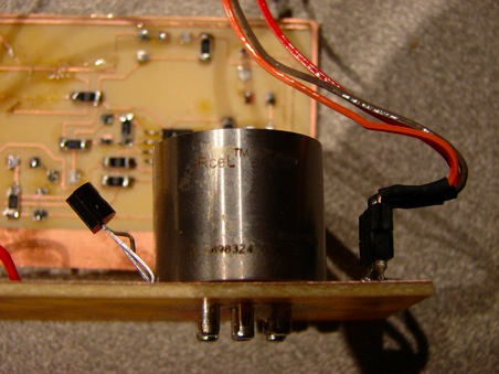
The IrCel amplification board required the use of cam.py and the Modela mill to create a through-hold board. This is because the IrCel has pins on the base which cannot be directly soldered (doing so would permanently damage the sensor). Accordingly, these pins must rest in socket connectors which must in installed as through-hold components. Power needed to be sourced from the Tiny45 driver board previously described.
This is how you make a through-hold PCB using Eagle and cam.py:
-
1.Create vias or through-holes as necessary in your .brd file
-
2.Power up CAM Processor
-
3.In the CAM Processor window, choose Open Job > Excellon
-
4.Save a .drd file
-
5.Go to the Modela mill and make sure to place a sacrificial board beneath your piece of FR4
-
6.Use cam.py to mill your .cmp file, but instead of clicking “auto” you MUST click “fixed”
-
7.Once you click “fixed,” numbers will appear in the x and y fields. To get registration correct, write down these numbers, add 0.9 inch to each of them, then use the command move to shift the mill to the proper location (x+0.9, y+0.9)
-
8.Mill your .cmp
-
9.DO NOT MOVE OR REMOVE YOUR BOARD
-
10.Use cam.py to open your .drd file
-
11.Again, click “fixed” and add 0.9 to the numbers which appear in the x and y fields. Use the command move to start the mill at this location, then make sure your z depth is set to 0.065 inches. Make certain there is enough play in the Modela’s starting endmill height to achieve this depth ...
Result: through-holes, just like the industry fab houses. See photo:
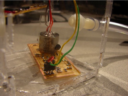
Enclosure Challenges
I decided to make a press-fit box to hold the system. Requirements included:
-
1.Airtight because otherwise it is difficult to make reliable readings
-
2.Ports for air inflow and air outflow, compatible with quarter-inch tubing
-
3.Port for data and power
-
4.Ability to open box up when necessary for reprogramming or upgrades
The press-fit box met all requirements apart from number 1. Even with the use of acrylic cement, I could not achieve an airtight system. An off-the shelf hermetically sealed unit would be preferable.
Final Result
The system worked and gave carbon dioxide output readings in real time. I noticed occasional strange behaviour whereby the 2Hz square wave would suddenly start jittering at more like 6Hz and lose all framing. This problem is intermittent and difficult to replicate.
The system I built is also functionally equivalent to a PC-based digital oscilloscope, with two channels of 10-bit data acquisition, an input range of 0V to 1.1V, and sampling at 1000Hz.